


ROIconnect is a freely available open-source plugin to EEGLAB for EEG data analysis. It allows you to perform linear and nonlinear functional connectivity analysis between regions of interest (ROIs) on source level. The results can be visualized in 2-D and 3-D. ROIs are defined based on popular fMRI atlases, and source localization can be performed through LCMV beamforming or eLORETA. Connectivity analysis can be performed between all pairs of brain regions using Coherence-based methods, Granger Causality, Time-reversed Granger Causality, Multivariate Interaction Measure, Maximized Imaginary Coherency, Phase-amplitude coupling, and other methods. This plugin is compatible with Fieldtrip, Brainstorm and NFT head models.
📚 Check out the following papers to learn about recommended methods and pipelines for connectivity experiments:
Pellegrini, F., Delorme, A., Nikulin, V., & Haufe, S. (2023). Identifying good practices for detecting inter-regional linear functional connectivity from EEG. NeuroImage, 120218. doi: 10.1016/j.neuroimage.2023.120218
Pellegrini, F., Nguyen, T. D., Herrera, T., Nikulin, V., Nolte, G., & Haufe, S. (2023). Distinguishing between- from within-site phase-amplitude coupling using antisymmetrized bispectra. bioRxiv 2023.10.26.564193. https://doi.org/10.1101/2023.10.26.564193
You can choose to access the core functions from the EEGLAB GUI. Experienced users can access additional utilities from the command line. If you do decide to run a function from the command line, please refer to the respective documentation provided in the code.
Code developed by Tien Dung Nguyen, Franziska Pellegrini, and Stefan Haufe, with EEGLAB interface, coregistration, 3-D visualization, and Fieldtrip integration performed by Arnaud Delorme.
First, install EEGLAB. Then, use menu item File > Manage EEGLAB extensions, select ROIconnect, and install. ROIconnect menu items are located in the Tools EEGLAB menu.
First, please make sure to have EEGLAB installed. Your project layout should look as follows.
eeglab/
├── functions/
├── plugins/
├── sample_data/
├── sample_locs/
├── tutorial_scripts/
└── /.../
The ROIconnect plugin should be installed in the plugins folder. The easiest way to do so is to simply clone our repository. Navigate to the plugins folder by typing.
cd <eeglab_install_location>/eeglab/plugins
Next, clone the repository.
git clone https://github.com/sccn/roiconnect.git
That's it! If you want to run the plugin, please start EEGLAB first. You may need to add EEGLAB to the MATLAB path. Some functions may require the additional installation of FieldTrip (lite or normal) and Brainmovie.
Why is this EEGLAB plugin not in the EEGLAB plugin manager? The plugin is beta. Once it is completed, it will be added to the EEGLAB plugin manager.
📌 test_pipes/ includes some test pipelines which can be used to get started.
The features of the toolbox are implemented in the following three main functions: pop_roi_activity, pop_roi_connect and pop_roi_connectplot. These functions have corresponding menus (documentation coming soon). For now, only the command line version of these functions is documented below.
You will need a leadfield matrix with an associated atlas to use ROIconnect. A leadfield matrix may be computed using the DIPFIT EEGLAB plugin (menu item Tools > Source localization using DIPFIT > Head model settings then Tools > Source localization using DIPFIT > Distributed source leadfield matrix). This leadfield matrix will be automatically recognized by ROIconnect.
pop_roi_activity asks for the following inputs: an EEG struct containing EEG sensor activitiy, a pointer to the headmodel and a source model, the atlas name and the number of PCs for the dimensionality reduction. In addition, this function also supports FOOOF analysis. Here is a command line example including FOOOF:
EEG = pop_roi_activity(EEG, 'leadfield',EEG.dipfit.sourcemodel,'model','LCMV','modelparams',{0.05},'atlas','LORETA-Talairach-BAs','nPCA',3, 'fooof', 'on', 'fooof_frange', [1 30]);The function performs source reconstruction by calculating a source projection filter and applying it to the sensor data. Power is calculated using the Welch method on the voxel time series and then summed across voxels within regions. To enable region-wise FC computation, the function applies PCA to the time series of every region. It then selects the n strongest PCs for every region. The resulting time series is stored in EEG.roi.source_roi_data, and power is stored in EEG.roi.source_roi_power.
Note that the function requires the data to be about 100 Hz, so it queries the user for resampling data. It also extracts data segment of 2 seconds I have changed the automatic epoch (segment) extraction for continuous data and also added a parameter for the number of epochs. Connectivity values vary with the length of the data so we always want to have the same number of epochs.
Say we set the number of epochs to 60 (2 second epochs). When you provide continuous data, then non-overlapping epochs are extracted. If there are more than 60, then the function selects 60 randomly. If there are less than 60, then the function increases the epoch overlap and try to extract data epochs again. If you provide data epochs as input (single trial ERPs), and there are not enough of them, they are bootstraped to reach the desired number.
pop_roi_connect accepts the following inputs: the EEG struct computed by pop_roi_activity and the names of the FC metrics. To avoid biases due to data length, we recommend keeping data length for all conditions constant. Thus, you can tell the function to estimate FC on time snippets of 60 s length (default) which can be averaged (default) or used as input for later statistical analyses. The following command line example asks the function to perform FC analysis on snippets using default values (explicitly passed as input parameters in this example).
EEG = pop_roi_connect(EEG, 'methods', { 'MIM', 'TRGC'}, 'snippet', 'on', 'snip_length', 60, 'fcsave_format', 'mean_snips');The function computes all FC metrics in a frequency-resolved way, i.e., the output contains FC scores for every frequency-region-region combination. The output of this function is stored in EEG.roi.<fc_metric_name>.
Note
Snippet analysis IS NOT equivalent to epoching. We discovered that the data length imposes a bias on the connectivity estimate. We therefore recommend keeping the data length (i.e. snippet length, default 60 s) constant across all experimental conditions that should be compared. This is most relevant for iCOH and MIM/MIC. By default, the snippet analysis is turned off (default:'snippet', 'off'). For more details, click here.
You can visualize power and FC in different modes by calling pop_roi_connectplot. Below, we show the results of a single subject from the real data example in [1]. You can find the MATLAB code and corresponding analyses here. The plots show power or FC in the left motor imagery condition. Due to the nature of the task, we show results in the 8 to 13 Hz frequency band but you are free to choose any frequency or frequency band you want.
📌 If any of the images are too small for you, simply click on them, and they will open in full size in another tab.
📍 Plotting is particularly optimized for PSD, MIM/MIC, and GC/TRGC.
If you wish to visualize power as a barplot only, please make sure to explicitly turn plotcortex off because it is turned on by default.
EEG = pop_roi_connectplot(EEG, 'measure', 'roipsd', 'plotcortex', 'off', 'plotbarplot', 'on', 'freqrange', [8 13]) % alpha band;

EEG = pop_roi_connectplot(EEG, 'measure', 'roipsd', 'plotcortex', 'on', 'freqrange', [8 13]);
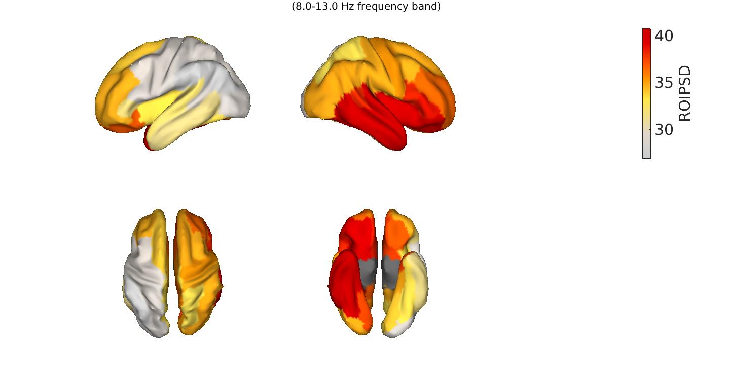
Again, if you do not wish to see the cortex plot, you should explicitly turn plotcortex off. Please click on the figure if you want to see it in full size.
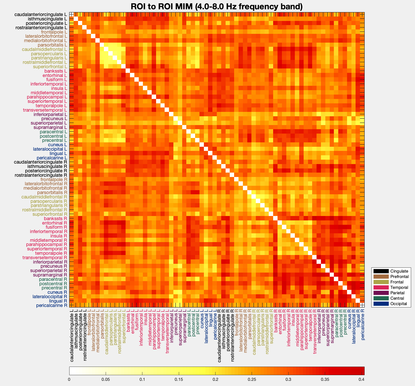
EEG = pop_roi_connectplot(EEG, 'measure', 'mim', 'plotcortex', 'off', 'plotmatrix', 'on', 'freqrange', [8 13]);

If you wish to group the matrix by hemispheres, you can do so by running the code below.
pop_roi_connectplot(EEG, 'measure', 'mim', 'plotcortex', 'off', 'plotmatrix', 'on', 'freqrange', [8 13], 'grouphemispheres', 'on');
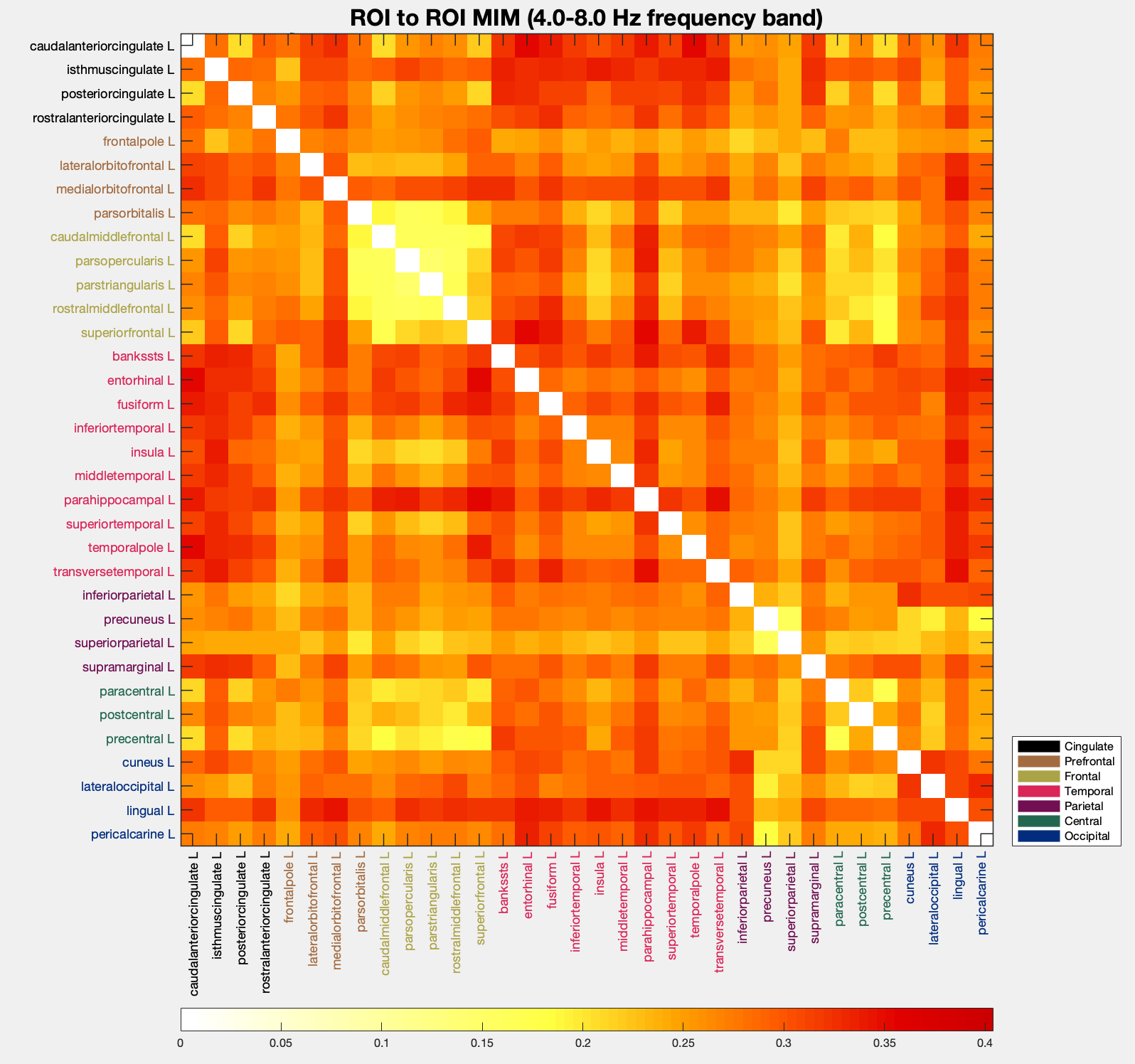
You can additionally filter by hemispheres and regions belonging to specific brain lobes. As an example, let us see how FC of the left hemisphere looks like.
pop_roi_connectplot(EEG, 'measure', 'mim', 'plotcortex', 'off', 'plotmatrix', 'on', 'freqrange', [8 13], 'hemisphere', 'left');
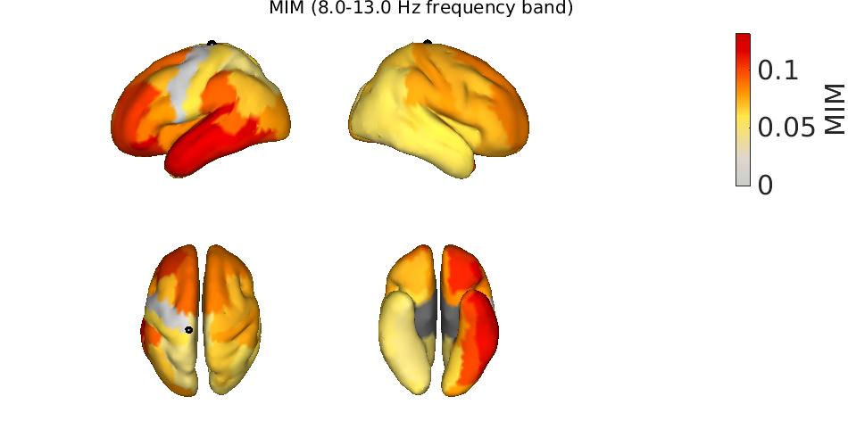
Here, the mean FC from all regions to all regions is visualized.
pop_roi_connectplot(EEG, 'measure', 'mim', 'plotcortex', 'on', 'freqrange', [8 13]);

Here, the FC of a seed region to all other regions is visualized.
pop_roi_connectplot(EEG, 'measure', 'mim', 'plotcortex', 'on', 'freqrange', [8 13], 'plotcortexseedregion', 49);
The ROIconnect plugin is compatible with EEGLAB STUDY framework. This means that if you have created a STUDY for group analysis, you can select ROIconnect menus to compute connectivity on a group of datasets. Once connectivity has been computed, there are two ways to aggregate results for ROIconnect at the group level. At this stage, both ways involve command line code. The simplest way is to run ROIconnect on all datasets and then gather the matrices and run statistics on them.
Assuming that you have computed connectivity (for example, the multivariate interaction measure) for all datasets and that for each subject, you have a dataset for condition 1 and a dataset for condition 2 (so in sequence, the first dataset is subject 1 condition 1, the second subject 1 condition 2, the third is subject 2 condition 1, etc, you could use the code:
% aggregate all subjects for each condition in one matrix
numSubject = length(ALLEEG)/2; % number os subjects
cond1 = zeros( [ size(ALLEEG(1).roi.MIM) numSubject] ); % dimensions are frequency x roi x roi x subject
cond2 = zeros( [ size(ALLEEG(1).roi.MIM) numSubject] );
for iSubj = 1:numSubject
	cond1(:,:,:,iSubj) = ALLEEG(((iSubj-1)*2+1)).roi.MIM; % get the MIM (multivariate interaction measure) for all odd datasets
	cond2(:,:,:,iSubj) = ALLEEG(((iSubj-1)*2+2)).roi.MIM; % get the MIM (multivariate interaction measure) for all even datasets
end

% compute statistics and plot
[t,df,p] = statcond({ cond1 cond2 }); % parametric here but you can also use permutations
[~,indAlpha] = min(abs(ALLEEG(1).roi.freqs - 10));
tAlpha = squeeze(t(indAlpha,:,:));
pAlpha = squeeze(pFdr(indAlpha,:,:));
figure; subplot(1,2,1); imagesc(tAlpha); title('t-value');
figure; subplot(1,2,2); imagesc(-log10(pAlpha)); title('p-value (0 for p=1; 1 for p=0.1; 2 for p=0.01 ...)');
% or replace matrix MIM in one of the dataset and plot using the ROIconnect menus or command line functions
Alternatively, to get ROIconnect data from an arbitrary study design (including 2-way ANOVA), you can use the powerful std_readdata function as outlined in the documentation of the eegstats plugin.
[~,condsMat] = std_readdata(STUDY, ALLEEG, 'customread', 'std_readeegfield', 'customparams', {{ 'roi', 'MIM' }}, 'ndim', 4, 'singletrials', 'on’);Then, proceed to use the compute statistics and plot as above (in this case condsMat = { cond1 cond2 }). For more information on how to create a STUDY and STUDY design, refer to the EEGLAB documentation.
The test folder of ROIconnect contains a variety of scripts. Of interest is the test_pipes/pipeline_connectivity.m which runs connectivity analysis on the EEGLAB tutorial dataset. This script can easily be modified to process other data.
[1] Pellegrini, F., Delorme, A., Nikulin, V., & Haufe, S. (2023). Identifying good practices for detecting inter-regional linear functional connectivity from EEG. NeuroImage, 120218. doi: 10.1016/j.neuroimage.2023.120218
[2] Pellegrini, F., Nguyen, T. D., Herrera, T., Nikulin, V., Nolte, G., & Haufe, S. (2023). Distinguishing between- from within-site phase-amplitude coupling using antisymmetrized bispectra. bioRxiv 2023.10.26.564193. https://doi.org/10.1101/2023.10.26.564193