Once you have simulated a PDE problem using FreeFem++ you may want to have a look at the results in Matlab or Octave. ffmatlib provides useful commands to create contour(), quiver() as well as patch() plots from FreeFem++ simulation results.
- Click on the button
Clone or download(above) and then on the buttonDownload ZIP - Unzip and change to the directory
demos. Run all FreeFem++ *.edp scripts to create example simulation data - Run the matlab
*.mdemo files with Matlab or Octave
Hint: The ffmatlib functions are stored in the folder ffmatlib. Use the addpath(path to ffmatlib) command to tell Matlab / Octave where the library functions are if you are working in a different directory.
capacitor_2d.m
capacitor_2d.edp
Screenshot: 3D Patch
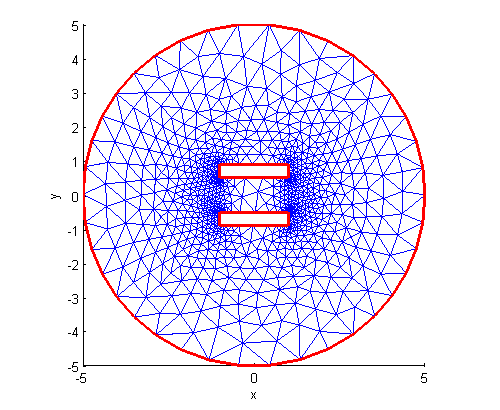
Screenshot: Mesh
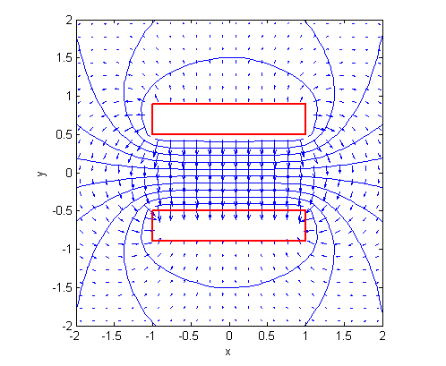
Screenshot: Contour and Quiver
Screenshot: 2D Patch with Mesh
Screenshot: Boundary and Labels
capacitor_3d.m
capacitor_3d.edp
Screenshot: 3D Slice
Screenshot: 3D Vector field
| Name | Description |
|---|---|
| ffpdeplot() | Creates contour(), quiver() as well as patch() plots from FreeFem++ 2D simulation data |
| ffinterpolate() | Interpolates PDE simulation data on a cartesian or curved meshgrid |
| fftri2grid() | Interpolates from a 2D triangular mesh to a 2D cartesian or curved grid (low level function) |
| ffpdeplot3D() | Creates cross-sections, quiver3() as well as boundary plots from FreeFem++ 3D simulation data |
| ffreadmesh() | Reads a FreeFem++ Mesh File into the Matlab / Octave workspace |
| ffreaddata() | Reads FreeFem++ Data Files into Matlab / Octave |
Is a function specially tailored to FreeFem++ that offers most of the features of the classic Matlab pdeplot() command. contour() plots (2D iso values), quiver() plots (2D vector fields) and patch() plots (2D map data) can be created as well as their combinations. In addition domain borders can be displayed and superimposed to the plot data.
ffpdeplot() can plot P0, P1, P1b and P2 - Lagrangian Element data.
[handles,varargout] = ffpdeplot(p,b,t,varargin)The FEM mesh is entered through its vertices, the boundary values and the triangles as provided by the FreeFem++ command savemesh(Th, "filename.msh"). The finite element connectivity data as well as the PDE simulation data is provided by the FreeFem++ macros ffSaveVh(Th, Vh, filename.txt) and ffSaveData(u, filename.txt). The contents of the points p, boundaries b and triangles t arguments are explained in the section ffreadmesh().
ffpdeplot() can be called with name-value pair arguments as per following table:
| Parameter | Value |
|---|---|
| 'VhSeq' | Finite element connectivity |
| FreeFem++ macro definition | |
| 'XYData' | PDE data used to create the plot |
| FreeFem++ macro definition | |
| 'XYStyle' | Coloring choice |
| 'interp' (default) | 'off' | |
| 'ZStyle' | Draws 3D surface plot instead of flat 2D Map plot |
| 'continuous' | 'off' (default) | |
| 'ColorMap' | ColorMap value or matrix of such values |
| 'off' | 'cool' (default) | colormap name | three-column matrix of RGB triplets | |
| 'ColorBar' | Indicator in order to include a colorbar |
| 'on' (default) | 'off' | 'northoutside' ... | |
| 'CBTitle' | Colorbar Title |
| (default=[]) | |
| 'ColorRange' | Range of values to adjust the colormap thresholds |
| 'off' | 'minmax' (default) | 'centered' | 'cropminmax' | 'cropcentered' | [min,max] | |
| 'Mesh' | Switches the mesh off / on |
| 'on' | 'off' (default) | |
| 'MColor' | Color to colorize the mesh |
| 'auto' (default) | RGB triplet | 'r' | 'g' | 'b' | |
| 'RLabels' | Meshplot of specified regions |
| [] (default) | [region1,region2,...] | |
| 'RColors' | Colorize regions with a specific color (linked to 'RLabels') |
| 'b' (default) | three-column matrix of RGB triplets | |
| 'Boundary' | Shows the domain boundary / edges |
| 'on' | 'off' (default) | |
| 'BDLabels' | Draws boundary / edges with a specific label |
| [] (default) | [label1,label2,...] | |
| 'BDColors' | Colorize boundary / edges with color (linked to 'BDLabels') |
| 'r' (default) | three-column matrix of RGB triplets | |
| 'BDShowText' | Shows the labelnumber on the boundary / edges |
| 'on' | 'off' (default) | |
| 'BDTextSize' | Size of labelnumbers on the boundary / edges |
| scalar value greater than zero | |
| 'BDTextWeight' | Character thickness of labelnumbers on the boundary / edges |
| 'normal' (default) | 'bold' | |
| 'Contour' | Isovalue plot |
| 'off' (default) | 'on' | |
| 'CStyle' | Contour plot style |
| 'solid' (default) | |
| 'CColor' | Isovalue color (can be monochrome or flat) |
| 'flat' | [0,0,0] (default) | RGB triplet, three-element row vector | 'r' | 'g' | 'b' | |
| 'CLevels' | Number of isovalues used in the contour plot |
| (default=10) | |
| 'CGridParam' | Number of grid points used for the contour plot |
| 'auto' (default) | [N,M] | |
| 'Title' | Title |
| (default=[]) | |
| 'XLim' | Range for the x-axis |
| 'minmax' (default) | [min,max] | |
| 'YLim' | Range for the y-axis |
| 'minmax' (default) | [min,max] | |
| 'ZLim' | Range for the z-axis |
| 'minmax' (default) | [min,max] | |
| 'DAspect' | Data unit length of the xy- and z-axes |
| 'off' | 'xyequal' (default) | [ux,uy,uz] | |
| 'FlowData' | Data for quiver plot |
| FreeFem++ point data | FreeFem++ triangle data | |
| 'FColor' | Color to colorize the quiver arrows |
| 'b' (default) | RGB triplet | 'r' | 'g' | |
| 'FGridParam' | Number of grid points used for quiver plot |
| 'auto' (default) | [N,M] |
The return value handles contains handles to the plot figures. The return value varargout contains references to the contour labels.
First of all the mesh, the finite element space sequence and the simulation data is loaded into the Matlab workspace:
[p,b,t]=ffreadmesh('capacitor_2d.msh');
[vh]=ffreaddata('capacitor_vh_2d.txt');
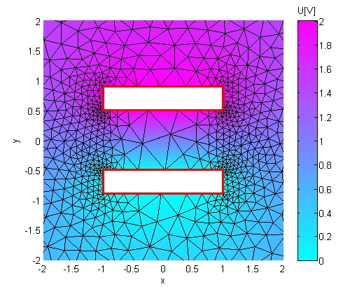
[u,Ex,Ey]=ffreaddata('capacitor_data_2d.txt');2D Patch Plot (2D map / density) without boundary:
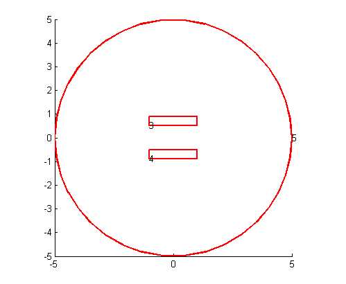
ffpdeplot(p,[],t,'VhSeq',vh,'XYData',u);Plot of the domain boundary:
ffpdeplot(p,b,t,'Boundary','on');2D Patch (2D Map or Density) Plot with boundary:
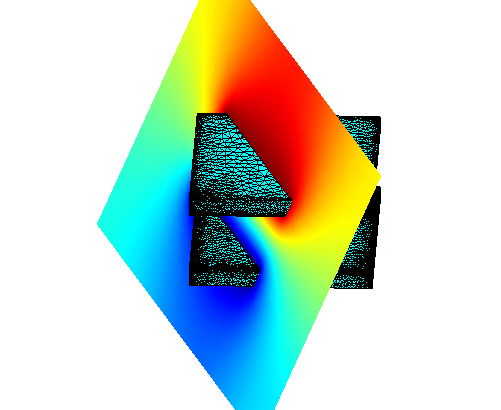
ffpdeplot(p,b,t,'VhSeq',vh,'XYData',u,'Mesh','on','Boundary','on');3D Surf Plot:
ffpdeplot(p,b,t,'VhSeq',vh,'XYData',u,'ZStyle','continuous');Contour Plot (isovalues):
ffpdeplot(p,b,t,'VhSeq',vh,'XYData',u,'Contour','on','Boundary','on');Quiver Plot (vector field):
ffpdeplot(p,b,t,'VhSeq',vh,'FlowData',[Ex, Ey],'Boundary','on');Interpolates from a 2D triangular mesh to a 2D cartesian or curved grid.
[varargout] = fftri2grid(x,y,tx,ty,varargin)
[varargout] = fftri2gridfast(x,y,tx,ty,varargin)fftri2grid computes the function values w1, w2, ... over a mesh grid defined by the arguments x, y from a set of functions u1, u2, ... with values given on a triangular mesh tx, ty. The interpolation values are computed using first order or second order approximating basis functions (P1, P1b or P2 - Lagrangian Finite Elements). The n-th function value wn is real if un is real and it is complex if un is complex. The mesh grid x, y can be cartesian or curved. fftri2grid returns NaNs when an interpolation point is outside the triangular mesh. fftri2gridfast.c is a runtime optimized mex implementation of the function fftri2grid.m. For more information see also Notes on MEX Compilation. fftri2grid() is a low level function and should not be called directly. To interpolate data, the wrapper function ffinterpolate.m should be used instead.
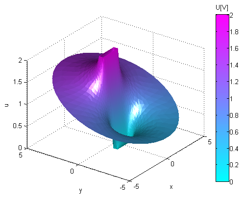
[p,b,t]=ffreadmesh('capacitor_2d.msh');
[vh]=ffreaddata('capacitor_vh_2d.txt');
[u,Ex,Ey]=ffreaddata('capacitor_data_2d.txt');
[~,pdeData]=convert_pde_data(p,t,vh,u');
[xmesh,~,ymesh,~]=prepare_mesh(p,t);
x=linspace(-5,5,500);
y=linspace(-5,5,500);
[X,Y]=meshgrid(x,y);
U=fftri2grid(X,Y,xmesh,ymesh,pdeData{1});
surf(X,Y,U,'EdgeColor','none');
view(3);Interpolates the real or complex valued multidimensional data u1, u2, ... given on a triangular mesh defined by the points p, triangles t and boundary b, onto a cartesian or curved grid defined by the arguments x, y.
[varargout] = ffinterpolate(p,[],t,vh,x,y,varargin)The n-th return value wn is real if the n-th input value un is real and it is complex if un is complex. ffinterpolate is a wrapper function that calls the library function fftri2grid. If Matlab/Octave finds a MEX - executable of fftri2gridfast.c within its search path the runtime optimized C-implementation is used instead of the matlab implementation fftri2grid.m. The contents of the p, b and t arguments are explained in the section ffreadmesh(). The content of u1, u2, ... is described in the section ffreaddata.
[p,b,t]=ffreadmesh('capacitor_2d.msh');
[vh]=ffreaddata('capacitor_vh_2d.txt');
[u,Ex,Ey]=ffreaddata('capacitor_data_2d.txt');
s = linspace(0,2*pi(),100);
Z = 3.5*(cos(s)+1i*sin(s)).*sin(0.5*s);
w = ffinterpolate(p,b,t,vh,real(Z),imag(Z),u);
plot3(real(Z),imag(Z),real(w),'g','LineWidth',2);
hold on;
ffpdeplot(p,b,t,'VhSeq',vh,'XYData',u,'ZStyle','continuous','ColorBar','off');Creates cross-sections, plots boundaries identified by a label and creates quiver3() plots from 3D simulation data. This function is still under construction.
ffpdeplot3D() can plot P0, P1 and P2 Lagrangian Finite Element - simulation data.
[] = ffpdeplot3D(p,b,t,varargin)The contents of the points p, boundaries b and triangles t arguments are explained in the section ffreadmesh(). Although the function can be run as Matlab code it is strongly recommended to build the MEX - executable from the file fftet2gridfast.c to improve execution speed. See also chapter Notes on MEX Compilation.
ffpdeplot3D() can be called with name-value pair arguments as per following table:
| Parameter | Value |
|---|---|
| 'VhSeq' | Finite element connectivity |
| FreeFem++ macro definition | |
| 'XYData' | PDE data used to create the plot |
| FreeFem++ data | |
| 'XYStyle' | Plot style for boundary |
| 'interp' (default) | 'noface' | 'monochrome' | |
| 'Boundary' | Shows the domain boundary / edges |
| 'on' (default) | 'off' | |
| 'BoundingBox' | Shows the bounding box of a slice |
| 'on' | 'off' (default) | |
| 'BDLabels' | Draws boundary / edges with a specific label |
| [] (default) | [label1,label2,...] | |
| 'Slice' | 3 point slicing plane definition |
| [] | three-column matrix of [x,y,z] triplets | |
| 'SGridParam' | Number of grid points used for the slice |
| 'auto' (default) | [N,M] | |
| 'Project2D' | View cross section in 2D |
| 'on' | 'off' (default) | |
| 'ColorMap' | ColorMap value or matrix of such values |
| 'cool' (default) | colormap name | three-column matrix of RGB triplets | |
| 'ColorBar' | Indicator in order to include a colorbar |
| 'on' (default) | 'off' | 'northoutside' ... | |
| 'CBTitle' | Colorbar Title |
| (default=[]) | |
| 'ColorRange' | Range of values to adjust the color thresholds |
| 'minmax' (default) | 'centered' | [min,max] | |
| 'Mesh' | Switches the mesh off / on |
| 'on' (default) | |
| 'FlowData' | Data for quiver3 plot |
| FreeFem++ point data | |
| 'FGridParam' | Number of grid points used for quiver3 plot at cross-section |
| 'auto' (default) | [N,M] | |
| 'FGridParam3D' | Number of grid points used for a spatial quiver3 plot |
| 'auto' (default) | [N,M,L] | |
| 'FLim3D' | Bounding box for a spatial quiver3 plot |
| 'auto' (default) | [xmin,xmax;ymin,ymax;zmin,zmax] | |
| 'FMode3D' | Arrow distribution choice |
| 'cartesian' (default) | 'random' |
First of all the mesh, the finite element space sequence and the simulation data is loaded into the Matlab workspace:
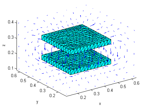
[p,b,t,nv,nbe,nt,labels]=ffreadmesh('cap3d.mesh');
[vh]=ffreaddata('cap3vh.txt');
[u]=ffreaddata('cap3dpot.txt');
[Ex,Ey,Ez]=ffreaddata('cap3dvec.txt');
The mesh is plot with a monochrome face color:
ffpdeplot3D(p,b,t,'XYZStyle','monochrome');In three dimensions boundaries can be buried inside a domain and therefore be invisible. If a particular label is given it is possible to display only the associated domain boundary. Following statement plots the boundaries/borders labeled with the numbers 30 and 31:
ffpdeplot3D(p,b,t,'BDLabels',[30,31],'XYZStyle','monochrome');The domain boundaries can be colored according to the PDE solution u:
ffpdeplot3D(p,b,t,'XYZData',u,'ColorMap','jet');Slices (cross-sections) for the volumetric data u can be created with the argument Slice. A slicing plane is defined by the parallelogram spanned by the three vertice points S1, S2 and S3. For example the following statement sequence shows two orthogonal cross-sections of the volumetric data u:
S1=[-0 0.375 0.0; ...
    0.375 0 0.0];
S2=[0.0 0.375 0.5; ...
    0.375 0 0.5];
S3=[0.75 0.375 0.0; ...
    0.375 0.75 0.0];
ffpdeplot3D(p,b,t,'VhSeq',vh,'XYZData',u,'Slice',S1,S2,S3,'Boundary','off','ColorMap','jet(200)', ...
            'SGridParam',[300,300],'BoundingBox','on')
A cross-section can also be viewed as 2D projection:
S1=[-0 0.375 0.0];
S2=[0.0 0.375 0.5];
S3=[0.75 0.375 0.0];
ffpdeplot3D(p,b,t,'VhSeq',vh,'XYZData',u,'Slice',S1,S2,S3,'SGridParam',[300,300], 'Project2D', 'on', ...
            'Boundary','off','ColorMap',jet(200),'ColorBar','on');
The following command plots a cross-section and additionally draws the mesh (facets are transparent):
ffpdeplot3D(p,b,t,'VhSeq',vh,'XYZData',u,'Slice',S1,S2,S3,'XYZStyle','noface','ColorMap','jet')A cross-section of three-dimensional vector fields can be plotted. The following example creates a quiver3() plot for a cross-section defined by the three points S1, S2, and S3:
ffpdeplot3D(p,b,t,'VhSeq',vh,'FlowData',[Ex,Ey,Ez],'Slice',S1,S2,S3,'Boundary','on','BoundingBox','on', ...
            'BDLabels',[30,31],'XYZStyle','monochrome');
If the parameter specification for the slice is omitted the vector field is displayed on a rectangular grid defined by the FGridParam3D and FLim3D parameters:
ffpdeplot3D(p,b,t,'VhSeq',vh,'FlowData',[Ex,Ey,Ez],'FGridParam3D',[8,8,5],'FLim3D', ...
[0.125,0.625;0.125,0.625;0.1,0.4],'BDLabels',[30,31],'XYZStyle','monochrome');Reads a FreeFem++ mesh file created by the FreeFem++ savemesh(Th,"2dmesh.msh") or savemesh(Th3d,"3dmesh.mesh") command into the Matlab/Octave workspace.
[p,b,t,nv,nbe,nt,labels] = ffreadmesh(filename)A mesh file consists of three parts:
- a mesh point list containing the nodal coordinates
- a list of boundary elements including the boundary labels
- list of triangles or tetrahedra defining the mesh in terms of connectivity
These three blocks are stored in the variables p, b and t respectively.
2D FreeFem++ (*.msh)
| Parameter | Value |
|---|---|
| p | Matrix containing the nodal points |
| b | Matrix containing the boundary edges |
| t | Matrix containing the triangles |
| nv | Number of points/vertices in the Mesh (Th.nv) |
| nt | Number of triangles in the Mesh (Th.nt) |
| nbe | Number of (boundary) edges (Th.nbe) |
| labels | Labels found in the mesh file |
3D INRIA Medit (*.mesh)
| Parameter | Value |
|---|---|
| p | Matrix containing the nodal points |
| b | Matrix containing the boundary triangles |
| t | Matrix containing the tetrahedra |
| nv | Number of points/vertices in the Mesh (nbvx, Th.nv) |
| nt | Number of tetrahedra in the Mesh (nbtet, Th.nt) |
| nbe | Number of (boundary) triangles (nbtri, Th.nbe) |
| labels | Labels found in the mesh file |
Read a mesh file into the Matlab/Octave workspace:
[p,b,t,nv,nbe,nt,labels]=ffreadmesh('capacitor_2d.msh');
fprintf('[Vertices nv:%i; Triangles nt:%i; Boundary Edges nbe:%i]\n',nv,nt,nbe);
fprintf('NaNs: %i %i %i\n',any(any(isnan(p))),any(any(isnan(t))),any(any(isnan(b))));
fprintf('Sizes: %ix%i %ix%i %ix%i\n',size(p),size(t),size(b));
fprintf('Labels found: %i\n',nlabels);
fprintf(['They are: ' repmat('%i ',1,size(labels,2)) '\n'],labels);Reads a FreeFem++ data file and / or finite element space sequence created with a FreeFem++ script to the Matlab/Octave workspace.
[varargout] = ffreadmesh(filename)Note: The data to be imported can be real or complex, integer or float. The data columns must be separated by a white space.
Read the FE-Space connectivity data and a set of data vectors into the Matlab/Octave workspace:
[vh]=ffreaddata('capacitor_vh_2d.txt');
[u,Ex,Ey]=ffreaddata('capacitor_data_2d.txt');In order to create a plot from a FreeFem++ simulation in Matlab / Octave
- The Mesh
- The FE-Space sequence in terms of connectivity
- The PDE simulation data
must be written into ASCII text files.
A FreeFem++ mesh can be exported using the FreeFem++ savemesh command:
savemesh(Th,"2d_mesh_file.msh");
savemesh(Th3d,"3d_mesh_file.mesh");
The FE-Space connectivity and the PDE simulation data can be written with the help of two macros located in the ffmatlib.idp file.
The following command saves the FE-Space sequence Vh:
ffSaveVh(Th,Vh,"vh.txt");The following command saves three data arrays into one text file:
ffSaveData3(u,Ex,Ey,"data.txt");In order to import the ASCII text files into the Matlab/Octave workspace the functions ffreadmesh and ffreaddata must be used.
Go into the folder ./ffmatlib/.
Octave:
Using gcc the MEX files are build with the commands:
mkoctfile --mex -Wall fftri2gridfast.c
mkoctfile --mex -Wall fftet2gridfast.c
Matlab before R2018:
With Microsoft Visual Studio the MEX files are build with the commands:
mex fftri2gridfast.c -v -largeArrayDims COMPFLAGS='$COMPFLAGS /Wall'
mex fftet2gridfast.c -v -largeArrayDims COMPFLAGS='$COMPFLAGS /Wall'
Matlab R2018 and later versions:
In Matlab release R2018 a new memory layout for complex numbers was introduced (i.e. the Interleaved Complex API). If you want to use the runtime optimized code on such a system use the files fftri2gridfast_matlab_R2018.c and fftet2gridfast_matlab_R2018.c. To compile these files on Windows with a gcc (mingw) compiler rename the two files and build the MEX executables with the commands:
setenv('MW_MINGW64_LOC','enter path to the mingw compiler');
mex -R2018a fftri2gridfast.c
mex -R2018a fftet2gridfast.c
It should be emphasized that the responsiveness of the plots is highly dependent on the degree of freedom of the PDE problem and the capabilities of the graphics hardware. For larger problems (lots of thousand of vertices), a dedicated graphics card should be used rather than an on board graphics. Hardware acceleration should be used extensively. Some notes on trouble shooting and tweaking:
If get(gcf,'RendererMode') is set to auto Matlab/Octave will decide on its own which renderer is the best for the current graphic task.
get(figure_handle,'Renderer')returns the current figure() rendererset(figure_handle,'Renderer','OpenGL')forces a figure() to switch to OpenGLset(figure_handle,'Renderer','painters')forces a figure() to switch to vector graphics
Generally OpenGL can be considered to be faster than painters. To get an OpenGL info type opengl info within Matlab. Ensure the line Software shows false otherwise OpenGL will run in software mode. If hardware-accelerated OpenGL is available on the system, the modes can be changed manually using the opengl software and opengl hardware commands. My personal experience is that Matlab R2018 runs much fastern than R2013.
Many thanks to David Fabre (StabFEM) for feature and implementation suggestions and code review.
GPLv3+
Have fun ...