Introduction

Introduction
How to setup the project
How to use the project
Understanding the Assignment
Designer Details
License

Introduction

The aim of the assignment is meant to get a better understanding of basic concepts of Robotics using tools like ROS2 Humble Hawksbill, Gazebo Sim, RVIZ and MathWorks® MATLAB The final project is divided into three seperate assignments:

Assignment 1: Build Model URDF, Forward Kinematics Node and Inverse Kinematics Node.
1. Setup the dynamically accurate model of robot in Gazebo by editing the model URDF.
2. Calculate the DH Parameters of the Robot to build a node that:
  1. Subscribes to the joint states of the robot and calculates the Pose of the robot by using Forward Kinematics.
  2. Publishes the Pose of the Robot to a new topic using a publisher.
3. Create an Inverse Kinematics Calculation Node that:
  1. Uses a custom service to take input of the (x,y,z) coordinates of the robot end-effector.
  2. Calculate the Joint States from the end-effector position and return it as a response to the service.
Assignment 2: Build a node to control Joint States.
1. Create a node that takes Reference Values for Joint Position as input through a service.
2. Build a Proportional-Derivative Controller that takes the current Joint States and Reference joint state to publish the control torque values to the /forward_effort_controller/commands topic.
3. Ensure that the model reaches the reference joint states in Gazebo.
Assignment 3: Build a node to control Joint or End-Effector Velocity.
1. Create a node with 2 services:
  1. Service 1 takes Joint Velocity as input to convert it to End-Effector Velocity as output.
  2. Service 2 takes End-Effector Velocity as input to convert it to Joint Velocity as ouput.
2. Based on the input, build a Proportional-Derivative controller that takes the current Joint Velocity and the Reference Joint Velocity to publish the torque values to the forward_effort_controller/commands topic.
3. Ensure that the model reaches the desired end-effector or joint velocity in Gazebo.

🗒 Note: This project is designed on Ubuntu 22.04 LTS and not tested on any other platforms

⚠ Warning: Remember, If anything doesnt work as it is supposed to, just use the rules of IT. Close it and restart it again 😃

How to setup the project

Install ROS2 Humble Hawksbill

Set locale

Make sure you have a locale which supports UTF-8. If you are in a minimal environment (such as a docker container), the locale may be something minimal like POSIX. We test with the following settings. However, it should be fine if you’re using a different UTF-8 supported locale.

locale  # check for UTF-8

sudo apt update && sudo apt install locales
sudo locale-gen en_US en_US.UTF-8
sudo update-locale LC_ALL=en_US.UTF-8 LANG=en_US.UTF-8
export LANG=en_US.UTF-8

locale  # verify settings

Setup Sources

You will need to add the ROS 2 apt repository to your system.

First ensure that the Ubuntu Universe repository is enabled.

sudo apt install software-properties-common
sudo add-apt-repository universe

Now add the ROS 2 GPG key with apt.

sudo apt update && sudo apt install curl
sudo curl -sSL https://raw.githubusercontent.com/ros/rosdistro/master/ros.key -o /usr/share/keyrings/ros-archive-keyring.gpg

Then add the repository to your sources list.

echo "deb [arch=$(dpkg --print-architecture) signed-by=/usr/share/keyrings/ros-archive-keyring.gpg] http://packages.ros.org/ros2/ubuntu $(. /etc/os-release && echo $UBUNTU_CODENAME) main" | sudo tee /etc/apt/sources.list.d/ros2.list > /dev/null

Install ROS 2 Packages

Update your apt repository caches after setting up the repositories.

sudo apt update

ROS 2 packages are built on frequently updated Ubuntu systems. It is always recommended that you ensure your system is up to date before installing new packages.

sudo apt upgrade

Desktop Install (Recommended): ROS, RViz, demos, tutorials.

sudo apt install ros-humble-desktop -y

Environment Setup

Sourcing the setup script

Set up your environment by sourcing the following file.

echo "source /opt/ros/humble/setup.bash" >> ~/.bashrc

Extra steps just to ensure colcon is properly installed

The ROS project hosts copies of the Debian packages in their apt repositories.

sudo sh -c 'echo "deb [arch=amd64,arm64] http://repo.ros2.org/ubuntu/main `lsb_release -cs` main" > /etc/apt/sources.list.d/ros2-latest.list'
curl -s https://raw.githubusercontent.com/ros/rosdistro/master/ros.asc | sudo apt-key add -

After that you can install the Debian package which depends on colcon-core as well as commonly used extension packages (see setup.cfg).

sudo apt update
sudo apt install python3-colcon-common-extensions

Gazebo Installation Tutorials

In this tutorial we will install Gazebo 11 and all its supporting files that will aid us in robot simulation.

Gazebo

Use the following commands to install Gazebo and its supplementry files

sudo sh -c 'echo "deb http://packages.osrfoundation.org/gazebo/ubuntu-stable `lsb_release -cs` main" > /etc/apt/sources.list.d/gazebo-stable.list'
wget https://packages.osrfoundation.org/gazebo.key -O - | sudo apt-key add -

Once this is done, update using and make sure it runs without any errors

sudo apt-get update

Now install Gazebo using

sudo apt-get install gazebo libgazebo-dev

You can check your installation by running this in a new terminal

gazebo

Gazebo ROS 2 packages

To use Gazebo with ROS2, there are certain packages that need to be installed

sudo apt install ros-humble-gazebo-ros-pkgs

Now we will install simulated robot controllers

sudo apt-get install ros-humble-ros2-control ros-humble-ros2-controllers
sudo apt-get install ros-humble-gazebo-ros2-control ros-humble-xacro
sudo apt-get install ros-humble-joint-state-publisher ros-humble-joint-state-publisher-gui

Now your system is ready to simulate any robot.

Spawn rrbot in Gazebo

Before doing colcon build we have to install some dependencies for the package to function correctly. Run the following commands in terminal

sudo apt install python3-pip
sudo pip3 install transforms3d

These are optional steps just to make sure everything is alright:

Please find the zipped package that has one of many ways to spawn an URDF in Gazebo using ROS2. The unedited files can be found in the directory:

/Resources/Group Project 1/rrbot_simulation_files.zip
Extract the package to your /src.

Once you have successfully installed all the required packages, find the supporting zip file that contains rrbot simulation files.

RRBOT:

That zip file contains 2 packages:

rrbot_description: This package contains the description files for the rrbot such as its urdf, gazebo plugins, ros2 control definitions etc. Xacro has been used instead of URDF to keep the description more modular, you will find that the main file rrbot.urdf.xacro includes a bunch of different files, so you don't have to deal with a very large file. The important files for us are rrbot.gazebo.xacro and rrbot.ros2_control.xacro, these contains the configuration for ROS2 Control. Visit this link for understanding how to configure ros2 control for your robot: https://github.com/ros-controls/gazebo_ros2_control
rrbot_gazebo: This package launches the actual simulation environment. The gazebo_controllers.yaml file in config helps us define what kind of controller we want to use, here we are using a forward_command_controller that just takes the command and applies it as it is, we have selected position as the command interface, i.e. we will control the position of the joints, reset all will be calculated by the controller. We can also use velocity or effort (torque) as the command interface. The state interfaces is what kind of feedback we will receive from JointStateBroadcastser, here we are taking position, velocity and effort feedbacks from the robot. JointStateBroadcaster is a different type of controller, it basically reads the current joint states from simulation environment and publishes it on the topic /joint_states.

The launch folder contains a launch file rrbot_world.launch.py which will be used to launch every thing, gazebo simulation environment, controller manager for ros2 control, robot state publisher.

Simulation

In the main folder run the following commands:

colcon build --symlink-install
. install/setup.bash

As we are using some gazebo plugins for camera, we need to source the gazebo setup bash file too

echo ". /usr/share/gazebo/setup.bash" >> ~/.bashrc

Now open a new terminal to launch rrbot in gazebo and run

ros2 launch rrbot_gazebo rrbot_world.launch.py

This should result in a new Gazebo window popping up with rrbot spawned, Now if you do ros2 topic list, you will be able to see a bunch of different topics /joint_states : This topic will have the robot's current state, i.e. position, velocity and efforts of each joint /forward_position_controller/commands : This is the control topic, this will be used to control the robot joints /camera1/image_raw : On this topic the robot will publish the camera feed, to visualize what the camera is seeing we can use rviz2.

🗒 Note: This can also result in your system getting hanged for a few minutes, this is just a first time thing and please don't kill the node if this happens, average hang-time is around 2-3 mins, if it goes above 10 mins kill the launch file.

PlotJuggler

Plot Juggler is a tool used for visualizing the topics with data for plotting.

Installation of Plot Juggler is pretty simple. Since we are using ROS2 Humble, we will install for the same edition of ROS.

Install the Plot Juggler using the command:

sudo apt-get install ros-humble-plotjuggler-ros

And we are all done with Plot Juggler Installation.

How to use the project

Assignment 1

Compile the project by using the command:
```
colcon build
```

Forward Kinematics Node

Launch the RVIZ model in a new terminal using:
```
ros2 launch rrbot_description view_robot.launch.py
```
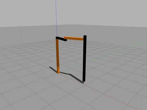
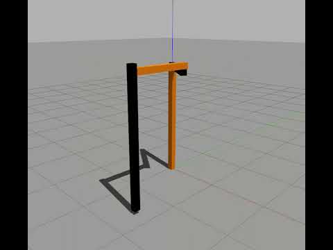
This will launch a Rviz windows which shows the robot model along with a a small window titled Joint State Publisher with three sliders to control three joints.
1. Rviz Model Window:

Joint Publisher Model:

In a new Terminal, Launch the Forward Kinematics node using:
```
ros2 run rrbot_gazebo fkin_publisher
```
The Node will take the Joint States from the topic /joint_states in the format sensor_msgs::msg::JointState

The Calculated Pose is published on the topic /forward_position_controller/commands in format std_msgs::msg::Float64MultiArray
In a new Terminal, Echo the Forward Kinematics Topic using
```
ros2 topic echo /forward_position_controller/commands
```
The output data will be displayed as follows:

The x coordinates is displayed at line 4.

The y coordinates is displayed at line 8.

The z coordinates is displayed at line 12.

Move around the sliders in the Joint State Publisher Window to see the End Effector Position change.

Inverse Kinematics Node

The Inverse Kinematics Node works on a server service node setup. The user can type the end-effector pose after launching the server node and request node to calculate the Joint States using a Service Call.

In a new terminal (You can close all other terminals if you wish to), Launch the Inverse Kinematics Server Node using:
```
ros2 run rrbot_gazebo ikin_publisher
```
In a new terminal launch the service using
```
ros2 service call /inverse_kinematics custom_interfaces/srv/FindJointStates "{x: 1, y: 0, z: 2}"
```
Change the end effector position by changing the values for (x,y,z).

The service Call will return the output in following format:

The service results two sets of possible response:

$(q_{11}, q_{21}, q_{31})$
$(q_{12}, q_{22}, q_{32})$

Assignment 2

Compile the project by using the command:
```
colcon build
```
Launch RRBOT in Gazebo using:
```
ros2 launch rrbot_gazebo rrbot_world.launch.py
```
This will launch the Gazebo Window with the RRBOT spawned.

Joint Position Control Node

Launch the Joint Control Node using:
```
ros2 run rrbot_gazebo joint_effort_control
```
The control strategy used for the Joint Control Strategy is PD Control. The system is broken down into individual joints where each joint has it's own control system. This strategy divides the whole system into 3 individual SISO System allowing us to tune Kp and Kd parameters individually.

$$u = -K_{p}*e - K_{d}\dot{e}$$

where:
- $e$ is position error: $e = \theta_{r} - \theta$
- $\dot{e}$ is rate of change of error: $\dot{e} = \frac{e_{t}-e_{t-\delta{t}}}{\delta{t}}$
Call the Joint Control service using:
```
ros2 service call /joint_state_controller custom_interfaces/srv/SetJointStates '{rq1: 1, rq2: 2, rq3: 2}'
```
Change the Joint States by trying different values for (rq1,rq2,rq3)

Right Click the Video below and open in new tab to see an example

Echo the topic to see the reference Joint Position:
```
ros2 topic echo /reference_joint_states/commands
```
We can visualize the efforts and joint states using PlotJuggler.

Launch Plot Juggler using the following:
```
ros2 run plotjuggler plotjuggler
```
Once the plot Juggler is launched, configure the system to view the joint data as follows:
1. Set the Streaming Tab for ROS2 Topic Subscriber and Buffer to 60 and press Start Button as shown:

After pressing the Start Button a new window will pop up with all the available topics labelled Select ROS messages

Select the Following three topics from list:
1. /forward_effort_controller/commands
2. /joint_states
3. /reference_joint_states/commands
Right Click on the tab1 canvas and Select Split Horizontally twice so you get a layout as shown below:

Drag and Drop the Following Topics in each Canvas from the Publishers Tab:
1. Canvas 1:
  1. /forward_effort_controller/commands/data.0
  2. /joint_states/joint1/position
  3. /joint_states/joint1/velocity
  4. /reference_joint_states/commands/data.0
2. Canvas 2:
  1. /forward_effort_controller/commands/data.1
  2. /joint_states/joint2/position
  3. /joint_states/joint2/velocity
  4. /reference_joint_states/commands/data.1
3. Canvas 3:
  1. /forward_effort_controller/commands/data.2
  2. /joint_states/joint3/position
  3. /joint_states/joint3/velocity
  4. /reference_joint_states/commands/data.2
The complete setup for visualization should look as below:

Assignment 3

Compile the project by using the command:
```
colcon build
```
Launch RRBOT in Gazebo using:
```
ros2 launch rrbot_gazebo rrbot_world.launch.py
```
This will launch the Gazebo Window with the RRBOT spawned.

Velocity Control Node

Launch the Velocity Control Node using:
```
ros2 run rrbot_gazebo end_eff_vel_control
```
The control strategy used for the Velocity Control Strategy is PD Control. The system is broken down into individual joints where each joint has it's own control system. This strategy divides the whole system into 3 individual SISO System allowing us to tune Kp and Kd parameters individually.

$$u = -K_{p}*e - K_{d}\dot{e}$$

where:
- $e$ is velocity error: $e = \dot{\theta_{r}} - \dot{\theta}$
- $\dot{e}$ is rate of change of error: $\dot{e} = \frac{e_{t} - e_{t-\delta{t}}}{\delta{t}}$
Velocity Control can be done in two way:
1. Joint Velocity Control: Here, the velocity of joint is directly controlled and the end effector moves accordingly
```
ros2 service call /joint_velocity_service custom_interfaces/srv/SetJointVelocity "{vq1: 1, vq2: 0, vq3: 0}"
```
1. End Effector Velocity Control: Here, the velocity of End Effector is set and accordingly the Robot Joint Velocity is calculated.
```
ros2 service call /end_effector_velocity_service custom_interfaces/srv/SetEndEffectorVelocity "{vx: 1, vy: 0, vz: 0}"
```
Right Click the Video below and open in new tab to see an example

We can visualize the efforts and joint states using PlotJuggler. Launch Plot Juggler using the following:
```
ros2 run plotjuggler plotjuggler
```
Once the plot Juggler is launched, configure the system to view the joint data as follows:
1. Set the Streaming Tab for ROS2 Topic Subscriber and Buffer to 60 and press Start Button as shown:

After pressing the Start Button a new window will pop up with all the available topics labelled Select ROS messages

Select the Following three topics from list:
1. /forward_effort_controller/commands
2. /joint_states
3. /reference_velocities/end_effector
4. /reference_velocities/joints
Right Click on the tab1 canvas and Select Split Horizontally twice so you get a layout as shown below:

Drag and Drop the Following Topics in each Canvas from the Publishers Tab:
1. Canvas 1:
  1. /forward_effort_controller/commands/data.0
  2. /joint_states/joint1/velocity
  3. /reference_velocities/end_effector/data.0
  4. /reference_velocities/joints/data.0
2. Canvas 2:
  1. /forward_effort_controller/commands/data.1
  2. /joint_states/joint2/velocity
  3. /reference_velocities/end_effector/data.1
  4. /reference_velocities/joints/data.1
3. Canvas 3:
  1. /forward_effort_controller/commands/data.2
  2. /joint_states/joint3/velocity
  3. /reference_velocities/end_effector/data.2
  4. /reference_velocities/joints/data.2
The complete setup for visualization should look as below:

The setup would plot graphs as shown

Understanding the Assignment

Assignment 1: Forward Kinematics Node

position_publisher.cpp

This node is the Forward Kinematics Node. It takes Joint Position as input and calculates End Effector Pose using it.

Include Essential File Headers

#include <chrono>
#include <functional>
#include <memory>
#include <string>
#include <vector>
#include <math.h> /* round, floor, ceil, trunc */

#include "rclcpp/rclcpp.hpp"
#include "std_msgs/msg/float64_multi_array.hpp"
#include "sensor_msgs/msg/joint_state.hpp"

Generating a Forward Kinematics Publisher Node

rclcpp::spin(std::make_shared<FKin_Publisher>());

Define Robot Physical Parameters

std::double_t l1 = 1, l2 = 1, ao = 0.05, lb = 1;

Create a subscriber that recieves Joint States from /joint_states and publishes the Robot Pose to /forward_position_controller/commands.

rclcpp::Publisher<std_msgs::msg::Float64MultiArray>::SharedPtr fkin_publisher_;
rclcpp::Subscription<sensor_msgs::msg::JointState>::SharedPtr joint_state_subscriber_;

We need a publisher and subscriber for our operation.

fkin_publisher : This publisher is used to publish the calculated pose from the recieved joint states.
joint_state_subscriber : The subscriber subscribes to the /joint_states topic and the is binded to the callback function void topic_callback(...) const using the std::bind(&FKin_Publisher::topic_callback, this, _1) command.

FKin_Publisher() : Node("minimal_publisher"), count_(0)
{
   fkin_publisher_ = this->create_publisher<std_msgs::msg::Float64MultiArray>("/forward_position_controller/commands", 10);
   joint_state_subscriber_ = this->create_subscription<sensor_msgs::msg::JointState>("/joint_states", 10, std::bind(&FKin_Publisher::topic_callback, this, _1));
}

The callback function is called everytime the Joint State subscriber recieves new Joint Values.

void topic_callback(const sensor_msgs::msg::JointState::SharedPtr msg) const

The Joint Position is stored in a Vector array

std::vector<std::double_t> joint_states = {msg->position[0],msg->position[1],msg->position[2]};
std::cout << joint_states[0] << "," << joint_states[1] << "," << joint_states[2] << std::endl;

Pose $(T)$ is calculated using the joint states using the formula

$$T= \begin{bmatrix} cos(\theta_{1}+\theta_{2})&-sin(\theta_{1}+\theta_{2})&0&cos(\theta_{1}+\theta_{2})+0.9cos(\theta_{1})\\\ sin(\theta_{1}+\theta_{2})&cos(\theta_{1}+\theta_{2})&0&sin(\theta_{1}+\theta_{2})+0.9sin(\theta_{1})\\\ 0&0&1&d_{3}+2.1\\\ 0&0&0&1 \end{bmatrix}$$

std::double_t pose[4][4] =
   {
      {{cos(joint_states[1] + joint_states[0])},{-sin(joint_states[1] + joint_states[0])},{(0)},{cos(joint_states[1] + joint_states[0]) + (9 * cos(joint_states[0])) / 10},},
      {{sin(joint_states[1] + joint_states[0])},{cos(joint_states[1] + joint_states[0])},{(0)},{sin(joint_states[1] + joint_states[0]) + (9 * sin(joint_states[0])) / 10},},
      {{(0)},{(0)},{(1)},{2.1 - joint_states[2]},},
      {{(0)},{(0)},{(0)},{(1)},}
   };

A variable is created in Float64MultiArray format which is a 1D-vector with the information of how it should be structured to act as a multidimensional array. It is done by defining the width and height of the array as shown

std_msgs::msg::Float64MultiArray message;
message.layout.dim.push_back(std_msgs::msg::MultiArrayDimension());
message.layout.dim[0].label = "width";
message.layout.dim[0].size = 4;
message.layout.dim[0].stride = 4 * 4;
message.layout.dim[1].label = "height";
message.layout.dim[1].size = 4;
message.layout.dim[1].stride = 4;
message.layout.data_offset = 0;

In order to remove any garbage data, we first fill the message variable with null value.

message.data.clear();

We flatten the pose variable to be copied into the publishing variable and copy the data

std::vector<double_t> vec(16, 0);
for (size_t i = 0; i < 4; i++)
   for (size_t j = 0; j < 4; j++)
      vec[(i * 4) + j] = pose[i][j];
message.data = vec;

The data is published on the topic as set before.

RCLCPP_INFO(this->get_logger(), "Publishing...");
fkin_publisher_->publish(message);

Assignment 1: Inverse Kinematics Node

FindJointStates.srv

The task of the service file is to define the input and output data type of the service.

Here we take $x,y,z$ as input and return $q_{11},q_{12},q_{13},q_{21},q_{22},q_{23}$ as output. Both are of type float64. The input and output is seperated by --- between them.

float64 x
float64 y
float64 z
---
float64 q11
float64 q21
float64 q31
float64 q12
float64 q22
float64 q32

joint_state_publisher.cpp

Including with essential headers.

#include "custom_interfaces/srv/find_joint_states.hpp"
#include "rclcpp/rclcpp.hpp"
#include <bits/stdc++.h>
#include <math.h>
#include <memory>

The node with name inverse_kinematics_server is generated and the service with name inverse_kinematics is attached to it.

The service calls the void add(...) function when it is initiated.

std::shared_ptr<rclcpp::Node> node = rclcpp::Node::make_shared("inverse_kinematics_server");
rclcpp::Service<custom_interfaces::srv::FindJointStates>::SharedPtr service = node->create_service<custom_interfaces::srv::FindJointStates>("inverse_kinematics", &add);

We round the input $x,y,z$ coordinates to 2 decimal places first and store it in variables.

std::double_t x = round(request->x * 100) / 100; // x component of the end effector pose
std::double_t y = round(request->y * 100) / 100; // y component of the end effector pose
std::double_t z = round(request->z * 100) / 100; // z component of the end effector pose

We check for the values of $x,y,z$ where robot cannot reach or will face singularity. We quit the node if it is not possible to calculate the solution.

if (std::sqrt((x * x) + (y * y)) > 2)
{
   RCLCPP_ERROR(rclcpp::get_logger("rclcpp"), "XY Values out of Bound");
   solution_possible = false;
}
if (x == 0 && y == 0)
{
   RCLCPP_ERROR(rclcpp::get_logger("rclcpp"), "XY Values not reachable. Detected Singularity");
   solution_possible = false;
}
if (z > 2.1 || z < 0)
{
   RCLCPP_ERROR(rclcpp::get_logger("rclcpp"), "Z Value out of Bound");
   solution_possible = false;
}
if (!solution_possible)
   return;

We define the Robot Parameters

std::double_t lb = 2;   // length of the base of the robot
std::double_t l1 = 0.9; // length of first link
std::double_t l2 = 1;   // length of second link
std::double_t l3 = 2.2; // length of third link

We calculate the Joint Position using Geometrical Approach. This is done using the lambda function in cpp

std::double_t q1_1, q1_2, q2_1, q2_2;
std::double_t q3 = lb + 0.1 - z; // prismatic joint displacement

double cos_of_q2 = (pow(x, 2) + pow(y, 2) - pow(l1, 2) - pow(l2, 2)) / (2 * l1 * l2);
auto get_q2 = [=](bool is_positive, double cos_of_q2)
{ return atan2((is_positive ? 1 : -1) * sqrt(1 - pow(cos_of_q2, 2)), cos_of_q2); };
q2_1 = get_q2(true, cos_of_q2);
q2_2 = get_q2(false, cos_of_q2);
auto get_q1 = [=](double q2)
{ return atan2(y, x) - atan2(l2 * sin(q2), l1 + (l2 * cos(q2))); };
q1_1 = get_q1(q2_1);
q1_2 = get_q1(q2_2);

The calculated Joint Position is rounded to 2 decimal places before submitting the response

// allocating the joint values to the server response
response->q11 = round(q1_1 * 100) / 100;
response->q21 = round(q2_1 * 100) / 100;
response->q31 = round(q3 * 100) / 100;

response->q12 = round(q1_2 * 100) / 100;
response->q22 = round(q2_2 * 100) / 100;
response->q32 = round(q3 * 100) / 100;

Assignment 2: Joint Position Control

SetJointStates.srv

The task of the service file is to define the input and output data type of the service.

Here we take $q_{1},q_{2},q_{3}$ as input of type float64. The input and output is seperated by --- between them. Since we don't have any return for this service file, the output end is kept empty. The output is displayed directly in the terminal live as the position is being achieved.

float64 rq1
float64 rq2
float64 rq3
---

joint_effort_controller.cpp

Include the required header files.

#include <chrono>
#include <functional>
#include <memory>
#include <string>
#include <vector>
#include <math.h> /* round, floor, ceil, trunc */

#include "rclcpp/rclcpp.hpp"
#include "std_msgs/msg/float64_multi_array.hpp"
#include "sensor_msgs/msg/joint_state.hpp"
#include "custom_interfaces/srv/set_joint_states.hpp"

Initialize the joint_state_controller node first.

rclcpp::init(argc, argv);
auto node = std::make_shared<joint_state_controller>();
RCLCPP_INFO(rclcpp::get_logger("rclcpp"), "Starting Joint Effort Control.");

Switch the Gazebo Robot from Position Controller to Effort Controller.

Position Controller: Takes joint positions as input and calculate the efforts on its own to reach the desired position.

Effort Controller: Takes efforts as input and directly applies it to the Robot Joints.

system("ros2 run rrbot_gazebo switch_eff");
system("ros2 topic pub --once /forward_effort_controller/commands std_msgs/msg/Float64MultiArray 'data: [0,0,0]'");
rclcpp::spin(node);

The following components are created for our usage.

service_ : Generate a service with name joint_state_controller to recieve Target Joint Position from User. The service calls the recieve_reference_joint_position_from_service(...) function everytime user sends the value via service call.
joint_state_subscriber : Subscriber to read the joint states (position and velocity) published by the gazebo robot on /joint_states topic. The subscriber is binded to void calculate_joint_efforts(...) function which is called everytime the subscriber recieves joint states.
efforts_publisher : Publishes the calculated joint efforts to the topic /forward_effort_controller/commands so the gazebo robot can implement it.
reference_value_publisher : Takes the reference joint values from service_ and publishes it on topic /reference_joint_states/commands so that it can be used to plot on graph.

service_ = this->create_service<custom_interfaces::srv::SetJointStates>("joint_state_controller", std::bind(&joint_state_controller::recieve_reference_joint_position_from_service, this, _1));
joint_state_subscriber_ = create_subscription<sensor_msgs::msg::JointState>("/joint_states", 10, std::bind(&joint_state_controller::calculate_joint_efforts, this, _1));
efforts_publisher_ = create_publisher<std_msgs::msg::Float64MultiArray>("/forward_effort_controller/commands", 10);
reference_value_publisher_ = create_publisher<std_msgs::msg::Float64MultiArray>("/reference_joint_states/commands", 10);

This function is called when the user initiates a service call for a robot to reach a certain position. We have a constraint on Joint 3 because it is a prismatic joint. The prismatic joint cannot be extended more than $2.1m$ and be less than $0m$. Joint 1 and Joint 2 being revolute, have no such constraints and can rotate infintely.

If the recieved positions are within constraints, they are stored in reference_position variable.

The command_received variable is switched to true when service call is made.

void recieve_reference_joint_position_from_service(const std::shared_ptr<custom_interfaces::srv::SetJointStates::Request> request)
{
   command_received_ = true;
   if (request->rq3 > 2.1 || request->rq3 < 0)
   {
      RCLCPP_ERROR(rclcpp::get_logger("rclcpp"), "Joint State 3 not reachable");
      return;
   }
   reference_position = {request->rq1,request->rq2,request->rq3};
   RCLCPP_INFO(rclcpp::get_logger("rclcpp"), "Request (q1,q2,q3): ('%f','%f','%f')", reference_position[0], reference_position[1], reference_position[2]);
}

calculate_joint_efforts function though called everytime joint_state_subscriber recieves the joint states, yet it is only effective once the command_received variable changes to true.

🤔 I Know! There are much better solution that the one we have implemented. But yeah!! It is what it is! We couldn't think of a smarter solution at 3 AM in the morning!!

We store the current joint position, velocity and calculate error in position.

$$ e = \theta_{r} - \theta $$

Our joint motion direction are switched so we are using the inverted directions.

std::vector<std::double_t> joint_position = {msg->position[0],msg->position[1],msg->position[2]};
std::vector<std::double_t> joint_velocity = {msg->velocity[0],msg->velocity[1],msg->velocity[2]};
std::vector<std::double_t> error = {joint_position[0] - reference_position[0],joint_position[1] - reference_position[1],joint_position[2] - reference_position[2]};

Initial efforts are:

$$\tau_{1} = 0 N$$

$$\tau_{2} = 0 N$$

$$\tau_{3} = 9.8 N$$

$\tau_{3}$ is kept at 9.8N so that the prismatic joint can hold its position when the desired position is achieved. This is due to the fact that the object has mass of 1kg.

apply_joint_efforts = {0, 0, 9.8};

The values of applied torque is changed only if the current error is greater than the acceptable error.

if (abs(error[0]) > acceptable_error) // Joint 1
   apply_joint_efforts[0] = -(proportional_gain[0] * error[0]) - (derivative_gain[0] * joint_velocity[0]);
if (abs(error[1]) > acceptable_error) // Joint 2
   apply_joint_efforts[1] = -(proportional_gain[1] * error[1]) - (derivative_gain[1] * joint_velocity[1]);
if (abs(error[2]) > acceptable_error) // Joint 3
   apply_joint_efforts[2] = -(proportional_gain[2] * error[2]) - (derivative_gain[2] * joint_velocity[2]);

A Float64MultiArray type variable is created to store the applied torque values for publishing it.

std_msgs::msg::Float64MultiArray message;
message.data.clear();
message.data = apply_joint_efforts;

The recieved joint states from the service is copied in a variable to publish it via the reference states publisher.

std_msgs::msg::Float64MultiArray reference_joint_states;
reference_joint_states.data = reference_position;

The Control efforts and reference joint states are finally published to their respective topics.

reference_value_publisher_->publish(reference_joint_states);
efforts_publisher_->publish(message);

Design Assumptions:

Acceptable Error = $0.0001 m$
Proportional Derivative (PD) Gains:
- Joint 1 $(K_{p1},K_{d1}) = (15,17)$
- Joint 2 $(K_{p2},K_{d2}) = (9.5,9.5)$
- Joint 3 $(K_{p3},K_{d3}) = (491,60)$

The tuning gains are high for Joint 3 primarily due to the fact that the Joint 3 is prismatic and along the direction of gravitational force causing it to need additional force to counteract the gravity. Opposite to it, Joint 1 and Joint 2 are revolute and working in direction perpendicular to gravity, thus, being able to operate with lowered applied torque.

std::double_t acceptable_error = 0.0001f;
std::vector<std::double_t> proportional_gain = {15, 9.5, 491};
std::vector<std::double_t> derivative_gain = {17, 9.5, 60};

When user presses Ctrl+C to close the node, a final command is sent so that the applied torques for all controllers can be set to zeros. This allows for any other node to be capable of controlling the robot along with clearing the topic of /forward_effort_controller/commands which won't spam the topic unnecessarily.

rclcpp::shutdown();
system("ros2 topic pub --once /forward_effort_controller/commands std_msgs/msg/Float64MultiArray 'data: [0,0,0]'");

🥳 Ladies and Gentlemen!!
🥳 Hope you have a good day!!
🥳 We are all done with the project here!!

Designer Details

Designed for:
- Worcester Polytechnic Institute
- RBE 500: Foundation of Robotics - Final Project
Designed by:
- Parth Patel
- Cameron Schloer

License

This project is licensed under GNU General Public License v3.0 (see LICENSE.md).

Licensed under the GNU General Public License, Version 3.0 (the "License"); you may not use this file except in compliance with the License.

You may obtain a copy of the License at

https://www.gnu.org/licenses/gpl-3.0.en.html

Unless required by applicable law or agreed to in writing, software distributed under the License is distributed on an "AS IS" BASIS, WITHOUT WARRANTIES OR CONDITIONS OF ANY KIND, either express or implied. See the License for the specific language governing permissions and limitations under the License.

Name		Name	Last commit message	Last commit date
Latest commit History 57 Commits
Resources		Resources
Submissions		Submissions
src		src
.gitignore		.gitignore
LICENSE.md		LICENSE.md
README.md		README.md

License

parth-20-07/PID-based-SCARA-Robot-Position-and-Velocity-Control-And-Manipulation

Folders and files

Latest commit

History

Repository files navigation

Introduction

How to setup the project

Install ROS2 Humble Hawksbill

Environment Setup

Gazebo Installation Tutorials

Simulation

How to use the project

Assignment 1

Forward Kinematics Node

Inverse Kinematics Node

Assignment 2

Joint Position Control Node

Assignment 3

Velocity Control Node

Understanding the Assignment

Assignment 1: Forward Kinematics Node

position_publisher.cpp

Assignment 1: Inverse Kinematics Node

FindJointStates.srv

joint_state_publisher.cpp

Assignment 2: Joint Position Control

SetJointStates.srv

joint_effort_controller.cpp

Designer Details

License

About

Topics

Resources

License

Stars

Watchers

Forks

Languages