The notebook presented in this repository contains a walk through of the Vision Transformer model with illustrations.
The notebook contains a step-by-step implementation of the paper 'An Image is Worth 16x16 Words: Transformers for Image Recognition at Scale'.
For the interactive version, visit this Colab Notebook.
Vision Transformer
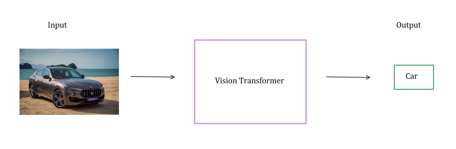
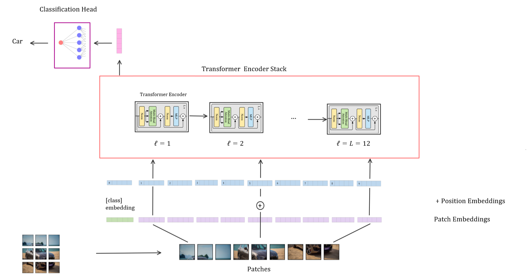
The Vision Transformer model takes an image and outputs the class of the image
The Vision Transformer model consists of the following steps:
-
Split an image into fixed-size patches
-
Linearly embed each of the patches
-
Prepend [class] token to embedded patches
-
Add positional information to embedded patches
-
Feed the resulting sequence of vectors to a stack of standard Transformer Encoders
-
Extract the [class] token section of the Transformer Encoder output
-
Feed the [class] token vector into the classification head to get the output
We start by splitting an image into fixed-size patches.

128 x 128 resolution image to 64 number of 16 x 16 resolution patches
We order the sequence of patches from top left to bottom right. After ordering, we flatten these patches.

We get a linear sequence with flattening
To generalize these steps for any image, we take an image with a resolution of height and width, and split it into a number of patches with a specified resolution that we call patch size, and flatten these patches.

We multiply the flattened patches with a weight matrix to obtain the embedding dimensionality that we want.

Multiply with a trainable linear projection to get embedding dimensionality, D = 768 in the paper
Now, as in the standard Transformer, we have a sequence of linear embeddings with a defined dimensionality.
We continue by prepending a [class] token to the patch embeddings. The [class] token is a randomly initialized learnable parameter that can be considered as a placeholder for the classification task.
The token gathers information from the other patches while flowing through the Transformer Encoders and the components inside the encoders. To be not biased toward any of the patches, we use the [class] token as a decoder, we apply the classification layer on the corresponding [class] token part of the output.
To describe the location of an entity in a sequence, we use Positional Encoding so that each position is assigned to a unique representation.
We add the positional embeddings with the intention of injecting location knowledge to the patch embedding vectors. Upon training, the position embeddings learn to determine the position of given image in a sequence of images.

Position embeddings are learnable parameters
With this final step, we obtain the embeddings that have all the information that we want to pass on. We feed this resulting matrix into a stack of Transformer Encoders.

Let’s dive into the structure of the Transformer Encoder.
The Transformer Encoder is composed of two main layers: Multi-Head Self-Attention and Multi-Layer Perceptron. Before passing patch embeddings through these two layers, we apply Layer Normalization and right after passing embeddings through both layers, we apply Residual Connection.

Transformer Encoder
Let’s look into the structure of the Multi-Head Self-Attention layer. The Multi-Head Self-Attention layer is composed by a number of Self-Attention heads running in parallel.
The Self-Attention mechanism is a key component of the Transformer architecture, which is used to capture contextual information in the input data. The self-attention mechanism allows a Vision Transformer model to attend to different regions of the input data, based on their relevance to the task at hand. The Self-Attention mechanism uses key, query and value concept for this purpose.
The key/value/query concept is analogous to retrieval systems. For example, when we search for videos on Youtube, the search engine will map our query (text in the search bar) against a set of keys (video title, description, etc.) associated with candidate videos in their database, then present us the best matched videos (values). The dot product can be considered as defining some similarity between the text in search bar (query) and titles in the database (key).
To calculate self-attention scores, we first multiply our input sequence with a single weight matrix (that is actually a uniform of three weight matrices). Upon multiplying, for each patch, we get a query vector, a key vector, and a value vector.

Key, Query and Value Matrices
We compute the dot products of the query with all keys, divide each by √ key dimensionality, and apply a softmax function to obtain the weights on the values. Softmax function normalizes the scores so they are all positive and add up to 1.
We then multiply the attention weights with values to get the Self-Attention output.

Weighted Values
Note that these calculations are done for each head separately. The weight matrices are also initialized and trained for each head separately.
In order to have multiple representation subspaces and to attend to multiple parts on an input, we repeat these calculations for each head and concatenate these Self-Attention outputs. After that, we multiply the result with a weight matrix to reduce the dimensionality of the output that grows in size with concatenation.

Obtaining results for each Attention Head, the number of heads is 12 in the paper

Getting Multi-head Self-Attention score
That is pretty much all there is to Multi-Head Self-Attention calculations.
Now, we will step into the other layer that is in the Transformer Encoder which is the Multi-Layer Perceptron.
Multi-Layer Perceptron is composed of two hidden layers with a Gaussian Error Linear Unit activation function in-between the hidden layers.
GELU, has a smoother, more continuous shape than the ReLU function, which can make it more effective at learning complex patterns in the data.

The hidden layers’ dimensionality is 3072 in the paper
Thus, we are done with the components of the Transformer Encoder.
We are left with one final component that makes up the Vision Transformer model which is the Classification Head.
If we continue from where we left off, after passing embedded patches through the Transformer Encoder stack, we achieved a Transformer Encoder output.
We extract the [class] token part of the Transformer Encoder output and pass it through a classification head to get the class output.
![[Class] Token of Output](https://cdn-images-1.medium.com/max/2394/1*RdCPl1XZGD72SXV_oR0Gcw.png)
[Class] Token of Output

Classification
Finally, by applying a Softmax function to the output layer, we obtain the probabilities of the class outputs.