Complex-Network-Analysis

NetLogo Model to generate and analyze complex networks and dynamics on them.

It works with NetLogo 6.0. Please read the Info Tab for instructions.

Complex Networks Toolbox

1. Introduction
2. The Interface
3. Scripts
4. Generators

* Erdős-Rényi Random Network
* Watts & Strogatz Small Worlds Networks
* Barabasi & Albert Preferential Attachtment
* Klemm and Eguílez Small-World-Scale-Free Network
* Geometric Network
* Spatially Clustered Network
* Grid
* Bipartite
* Edge Copying Dynamics

1. Global Measures
2. Utilities

* Layouts
* Compute Centralities
* Communities

1. Dynamics

* Page Rank
* Spread of infection/message
* Cellular Automata

1. Input/Output

* Save / Load GraphML
* Export Distributions

Introduction

This NetLogo model is a toy tool to launch experiments for Complex Networks.

It provides some basic commands to generate and analyze small networks by using the most common and famous algorithms (random graphs, scale free networks, small world, etc). Also, it provides some methods to test dynamics on networks (spread processes, page rank, cellular automata,...).

All the funtionalities have been designed to be used as extended NetLogo commands. In this way, it is possible to create small scripts to automate the generating and analyzing process in an easier way. Of course, they can be used in more complex and longer NetLogo procedures, but the main aim in their design is to be used by users with no previous experience on this language (although, if you know how to program in NetLogo, you can probably obtain stronger results).

In the next sections you can find some details about how to use it.

The Interface

Although the real power of the system is obtained via scripting, and it is its main goal, the interface has been designed to allow some interactions and facilitate to handle the creation and analysis of the networks. Indeed, before launching a batch of experiments is a good rule to test some behaviours by using the interface and trying to obtain a partial view and understanding of the networks to be analyzed... in this way, you will spend less time in experiments that will not work as you expect.

The interface has 3 main areas:

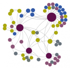
1. Network Representation: In the left side. It has a panel where the network is represented and it allows one only interaction, to inspect node information (when the button Inspect Node is pressed). Under this panel some widgets to manage the visualization properties are located: selected layout and parameters for it.
2. Measures Panel: In the right side. It contains a collection of plots where the several centralities are shown and some monitors with global information about the current network. The measures that are computed for every node are:

* Degree
* Clustering
* Betweenness
* Eigenvector
* Closeness
* Page-Rank

Scripts

Use scripts.nls to write your customized scripts. In order to acces this file, you must go to Code Tab and then choose ´scripts.nls´ from Included Files chooser. You can add as many aditional files as you want if you need some order in your experiments and analysis (load them with the __includes command from main file).

Remember that a script is only a NetLogo procedure, hence it must have the following structure:

to script-name
  ... 
  Commands
  ...
end

After defining your scripts, you can run them directly from the Command Center.

In the document you can find specific network commands that can be used to write scripts for creating and analyzing networks. In fact, this scripts can be written using any NetLogo command, but in this library you can find some shortcuts to make easier the process.

Some of the useful NetLogo commands you will probably need are:

• let v val : Create a new variable v and sets its value to val.
• set v val : Change the value fo the variable v to val.
• [ ] : Empty list, to store values in a repetition
• range x0 xf incx : Returns a ordered list of numbers from x0 to xf with incx increments.
• foreach [x1....xn] [ [x] -> P1...Pk ] : for each x in [x0 ... xn] it executes the comands P1 to Pk.
• repeat N [P1...Pk] : Repeat the block of commands P1 to Pk, N times.
• store val L : Store value val in list L.
• mean/max/min/sum L : Returns the mean/max/min/sum value of list L.
• print v : Print value of v in the Output.
• plotTable [x1...xn] [y1...yn] : Plot the points (x1,y1)...(xn,yn).

You can combine both to move some parameter in the creation/analysis of the networks. In the next example we study how the diameter of a Scale Free Network (built with Barabasi-Albert algorithm) changes in function of the size of the network:

foreach (range 10 1000 10)
[ [N] ->
    clear
    BA-PA N 2 1
    print diameter
]

For example, the next script will perform a experiment moving a parameter from 0 to 0.01 with increments of 0.001, and for every value of this parameter it will prepare 10 networks to compute their diameter.

to script5 
  clear 
  foreach (range 0 .01 .001)
  [ [p] ->
    print p
    repeat 10
    [
      clear 
      BA-PA 300 2 1
      ER-RN 0 p
      print diameter
    ]
  ]
end

From the Output we can copy/export the printed values and then analyze them in any other analysis software (R, Python, NetLogo, Excel, etc.)

Generators

The current generators of networks (following several algorithms to get different structures) are:

Erdős-Rényi Random Network:

In fact this is the Gilbert variant of the model introduced by Erdős and Rényi. Each edge has a fixed probability of being present (p) or absent (1-p), independently of the other edges.

N - Number of nodes, p - link probability of wiring

ER-RN N p

Watts & Strogatz Small Worlds Networks:

The Watts–Strogatz model is a random graph generation model that produces graphs with small-world properties, including short average path lengths and high clustering. It was proposed by Duncan J. Watts and Steven Strogatz in their joint 1998 Nature paper.

Given the desired number of nodes N, the mean degree K (assumed to be an even integer), and a probability p, satisfying N >> K >> ln(N) >> 1, the model constructs an undirected graph with N nodes and NK/2 edges in the following way:

1. Construct a regular ring lattice, a graph with N nodes each connected to K neighbors, K/2 on each side.
2. Take every edge and rewire it with probability p. Rewiring is done by replacing (u,v) with (u,w) where w is chosen with uniform probability from all possible values that avoid self-loops (not u) and link duplication (there is no edge (u,w) at this point in the algorithm).

N - Number of nodes, k - initial degree (even), p - rewiring probability

WS N k p

Barabasi & Albert Preferential Attachtment:

The Barabási–Albert (BA) model is an algorithm for generating random scale-free networks using a preferential attachment mechanism. Scale-free networks are widely observed in natural and human-made systems, including the Internet, the world wide web, citation networks, and some social networks. The algorithm is named for its inventors Albert-László Barabási and Réka Albert.

The network begins with an initial connected network of m_0 nodes.

New nodes are added to the network one at a time. Each new node is connected to m <= m_0 existing nodes with a probability that is proportional to the number of links that the existing nodes already have. Formally, the probability p_i that the new node is connected to node i is

         k_i
p_i = ----------
      sum_j(k_j)

where k_i is the degree of node i and the sum is made over all pre-existing nodes j (i.e. the denominator results in twice the current number of edges in the network). Heavily linked nodes ("hubs") tend to quickly accumulate even more links, while nodes with only a few links are unlikely to be chosen as the destination for a new link. The new nodes have a "preference" to attach themselves to the already heavily linked nodes.

N - Number of nodes, m0 - Initial complete graph, m - Number of links in new nodes

BA-PA N m0 m

Klemm and Eguílez Small-World-Scale-Free Network:

The algorithm of Klemm and Eguílez manages to combine all three properties of many “real world” irregular networks – it has a high clustering coefficient, a short average path length (comparable with that of the Watts and Strogatz small-world network), and a scale-free degree distribution. Indeed, average path length and clustering coefficient can be tuned through a “randomization” parameter, mu, in a similar manner to the parameter p in the Watts and Strogatz model.

It begins with the creation of a fully connected network of size m0. The remaining N−m0 nodes in the network are introduced sequentially along with edges to/from m0 existing nodes. The algorithm is very similar to the Barabási and Albert algorithm, but a list of m0 “active nodes” is maintained. This list is biased toward containing nodes with higher degrees.

The parameter μ is the probability with which new edges are connected to non-active nodes. When new nodes are added to the network, each new edge is connected from the new node to either a node in the list of active nodes or with probability μ, to a randomly selected “non-active” node. The new node is added to the list of active nodes, and one node is then randomly chosen, with probability proportional to its degree, for removal from the list, i.e., deactivation. This choice is biased toward nodes with a lower degree, so that the nodes with the highest degree are less likely to be chosen for removal.

N - Number of nodes, m0 - Initial complete graph, μ - Probability of connect with low degree nodes

KE N m0 μ

Geometric Network:

It is a simple algorithm to be used in metric spaces. It generates N nodes that are randomly located in 2D, and after that two every nodes u,v are linked if d(u,v) < r (a prefixed radius).

N - Number of nodes, r - Maximum radius of connection

Geom N r

Spatially Clustered Network:

This algorithm is similar to the geometric one, but we can prefix the desired mean degree of the network, g. It starts by creating N randomly located nodes, and then create the number of links needed to reach the desired mean degree. This link creation is random in the nodes, but choosing the shortest links to be created from them.

N - Number of nodes, g - Average node degree

SCM N g

Grid (2D-lattice):

A Grid of N x M nodes is created. It can be chosen to connect edges of the grid as a torus (to obtain a regular grid).

M - Number of horizontal nodes N - Number of vertical nodes t? - torus?

Grid N M t?

Bipartite:

Creates a Bipartite Graph with N nodes (randomly typed to P0 P1 families) and M random links between nodes of different families.

N - Number of nodes M - Number of links

BiP N M

Edge Copying Dynamics

The model introduced by Kleinberg et al consists of a itearion of three steps:

1. Node creation and deletion: In each iteration, nodes may be independently created and deleted under some probability distribution. All edges incident on the deleted nodes are also removed. pncd - creation, (1 - pncd) deletion.

2. Edge creation: In each iteration, we choose some node v and some number of edges k to add to node v. With probability β, these k edges are linked to nodes chosen uniformly and independently at random. With probability 1 − β, edges are copied from another node: we choose a node u at random, choose k of its edges (u, w), and create edges (v, w). If the chosen node u does not have enough edges, all its edges are copied and the remaining edges are copied from another randomly chosen node.

3. Edge deletion: Random edges can be picked and deleted according to some probability distribution.

Iter - Number of Iterations pncd - probability of creation/deletion random nodes k - edges to add to the new node beta - probability of new node to uniform connet/copy links pecd - probability of creation/deletion random edges

Edge-Copying Iter pncd k beta pecd

Global Measures

The global measures we can take from any network are:

Number-Nodes
Number-Links
Density
Average-Degree
Average-Path-Length
Diameter
Average-Clustering
Average-Betweenness, 
Average-Eigenvector, 
Average-Closeness, 
Average-Page-Rank
All

Some of them need to compute centralities before they can be used. If you choose All, ypu obtain a list with all the measures of the network.

You can print any of them in the Output Window:

Print measure

Utilities

Layouts

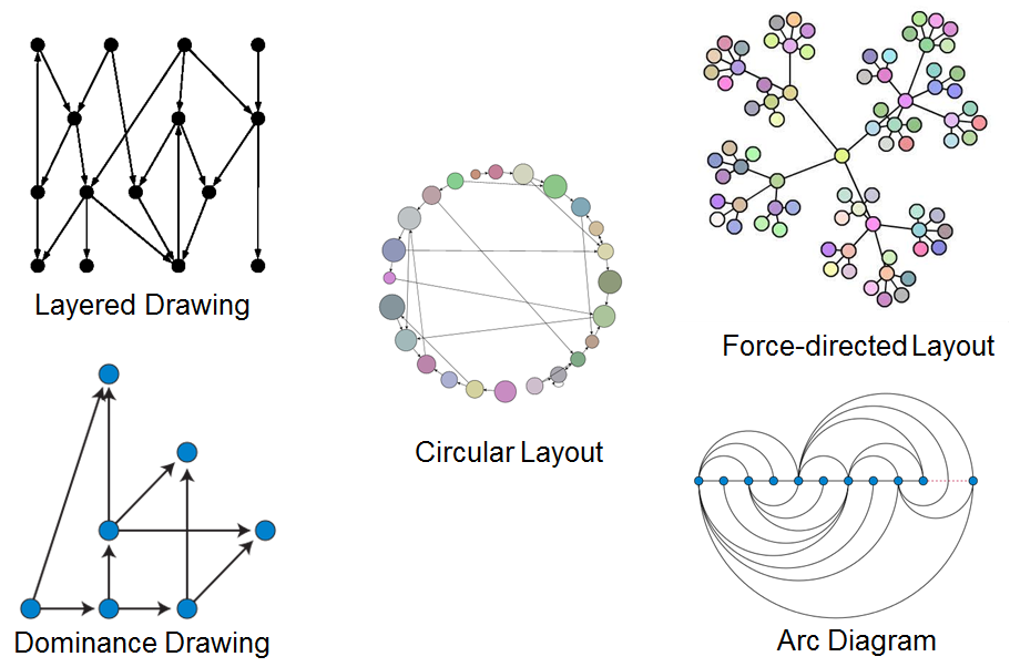
The system allows the following layouts:

circle
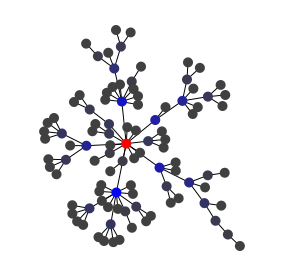
radial (centered in a max degree node)
tutte
spring (1000 iterations)
bipartite

To use it from a script:

layout type-string

For example:

layout "circle"

Compute Centralities

Current Centralities of every node:

Betweenness, 
Eigenvector, 
Closeness, 
Clustering, 
Page-Rank

The way to compute all of them is by executing:

compute-cantralities

Communities

Computes the communities of the current network using the Louvain method (maximizing the modularity measure of the network).

Dynamics

Page Rank

Applies the Page Rank diffusion algorithm to the current Network a number of prefixed iterations.

Iter - Number of iterations

PRank Iter

Rewire

Rewires all the links of the current Network with a probability p. For every link, one of the nodes is fixed, while the other is rewired.

p - probability of rewire every link

Rewire p

Spread of infection/message

Applies a spread/infection algorithm on the current network a number of iterations. It starts with a initial number of infected/informed nodes and in every step:

1. The infected/informed nodes can spread the infection/message to its neighbors with probability ps (independently for every neighbor).

2. Every infected/informed node can recover/forgot with a probability of pr.

3. Every recovered node can become inmunity with a probability of pin. In this case, he will never again get infected / receive the message, and it can't spread it.

N-mi - Number of initial infected nodes ps - Probability of spread of infection/message pr - Probability od recovery / forgotten pin - Probability of inmunity after recovering Iter - Number of iterations

Spread N-mi ps pr pin Iter

Cellular Automata

Discrete Totalistic Cellular Automata

The nodes have 2 possible values: on/off. In every step, every node changes its state according to the ratio of activated states.

Iter - Number of iterations pIn - Initial Probability of activation p0_ac - ratio of activated neighbors to activate if the node is 0 p1_ac - ratio of activated neighbors to activate if the node is 1

DiscCA Iter pIn p0_ac p1_ac

Continuous Totalistic Cellular Automata

The nodes have a continuous possitive value for state: [0,..]. In every step, every node changes its state according to the states of the neighbors:

s'(u) = p * s(u) + (1 - p) * avg {s(v): v neighbor of u}

Iter - Number of iterations pIn - Initial Probability of activation p - ratio of memory in the new state

ContCA Iter pIn p

Input/Output

Save GraphML / Load GraphML

Opens a Dialog windows asking for a file-name to save/load current network.

Save
Load

Export Distributions

You can export the several distributions of the measures for a single network:

export view

Where view can be any of the following:

Degree
Clustering
Betweenness
Eigenvector
Closeness
PageRank

The program will automatically name the file with the distribution name and the date and time of exporting.