Team doubleSpeak: Begum Kasap, Rishad Raiyan
This project aims to identify speakers by making use of mel-frequency cepstrum, vector quantization and LGB algorithm. Audio files are pre-processed in order to normalize their amplitudes and remove any silent portions. A Hamming window frame of size 256 is used to compute STFT. Frame increment is set to 256/3. 20 mel-filter banks are used to get 20 MFCC coefficients. A codebook is generated from training dataset using 20 MFCCs and 16 clusters. The Test dataset is compared against the codebook and the speakers are classified based on average distortion between test data samples and codebooks' centroids. A total of 11 audio files were provided for training and testing purposes. If we use all 11 audio files for training and testing, we achieved 100% accuracy from the provided training dataset and 81.82% accuracy from the provided test data set. If we use only 8 audio files for training and 11 audio files for testing, our algorithm can correctly reject 2/3 of new unknown skeapers and achieves 71.73% testing accuracy. Furthermore, we collected additional training and testing audio recordings from 3 different people. We achieved an accuracy of 100% on the new training dataset and 71.43% accuracy from the new test data set. The human performance accuracy is recorded as 62.5% (average between two human performances). Therefore, our model performs better than human benchmark.
After downloading the gitHub repo, you may run 'classifying_voices.mlx' to display the accuracies on different datasets (provided and new). This script also plots the time-domain plot and spectrums of training dataset before and after pre-processing. The MFCC coefficients (Cepstrum) as well as Mel-frequency filter bank are also plotted.
You may run 'VQ.m' to plot speaker's data samples and computed centroids in the codebook in a 2D MFCC space. MFCC-2 and MFCC-3 are chosen for these 2D plots.
The provided dataset for this project comprised of 11 speechfiles recorded by 11 distinc speakers saying 'Zero'. Each speachfile is named in format S{x}.wav where {x} is the ID of the speaker (x = 1...11). The speechfiles are located under /Data folder. We aim to train a voice model by creating a VQ codebook in the MFCC vector space for each speaker under 'training_data'. The codebook will contain information on voice characteristic of each (known) speaker. Next, we try identifying the speaker ID of speachfiles located under 'test_data'. In order to have a benchmark, we recorded how accurate humans can identify the speakers and took the average between two human separate performances. We recorded an accuracy of 62.5% as human performance.
Speech signals are quasi-stationary meaning that when examined with Short-Time Fourier Transform (STFT) with a sufficiently short frame (20.48 msec in this project) their frequency characteristics are mostly stationary. The variation of frequency characteristics over a long duration (>1/5 seconds) would reveal information on different sounds being produced. Although short-time spectral analysis is a good starting point to characterize speech signal it is not sufficient for the speaker recognition task. We compute Mel-Frequency Cepstrum Coefficients (MFCC) from the spectrums in order to parametrically represent speech signal. Since humans are good at recognizing speakers, MFCC's are based on the known variation of the human ear’s critical bandwidths with frequency. We use a Mel-Filter bank with 20 filters spaced linearly at low frequencies and logarithmically at high frequencies to capture the phonetically important characteristics of speech. In the end we have 20 MFCCs which are our features to be used in speaker identification. These steps are summarized in Figure B0 below. The steps described in this section are implemented under the function 'mfcc.m' present in this repo.
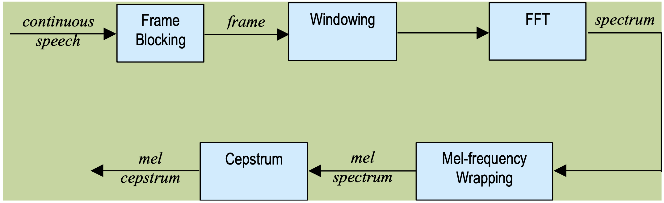
Figure B0: Block diagram of the MFCC processor
We first start by pre-processing the speechfiles. Figure B1 shows the time domain plot of unprocessed 11 speechfiles. One can notice that the speechfiles are long and we need to crop the beginning and end portions of the speach where the speaker is not talking. Also each speaker's voice has a different amplitude and different mean. For example, S9, S10 and S11 have a certain offset and does not have a mean of zero. We should normalize the amplitudes of the time-domain speaker data, by dividing by maximum absolute amplitude, so that our speaker identifier algorithm is robust against variations in volume of the speaker. We also remove the offset before normalizing.
 Figure B1: Time domain plots of raw speechfiles
Let's also take a look into the frequency content over time of unprocessed speechfiles. We use STFT to generate the spectrograms plotted in Figure B2. The speechfiles have a sampling rate of 12.5kHz. A Hamming window size of 256 samples/20.48 msec is used to generate the spectrograms. The Frame increment between windows is set to 1/3 of frame size. A window size of 256 samples was chosen because typical adult female voice frequency is from 165Hz to 255Hz and typical adult male voice frequency is from 85Hz to 180Hz. Therefore, we can have at least 49 samples (12.5kHz/255Hz) and at most 147 samples (12.5kHz/85Hz) within a period of any voice signal. When choosing the window size for STFT we need to make sure we have at least one or two periods of voice signals within a frame and 256 samples frame size is a good fit.
 Figure B2: Spectrograms of raw speechfiles
When we observe the spectrograms of the speechfiles we notice that most of the frequency content is at lower frequencies and the periodogram has high amplitude in time when the speaker starts speaking. We can remove the silent portions of the audio files by only keeping the data with a normalized amplitude of 0.02 (-34dB) or higher. Figure B3 shows the time-domain plots and figure B4 shows the spectrograms of the processed data.
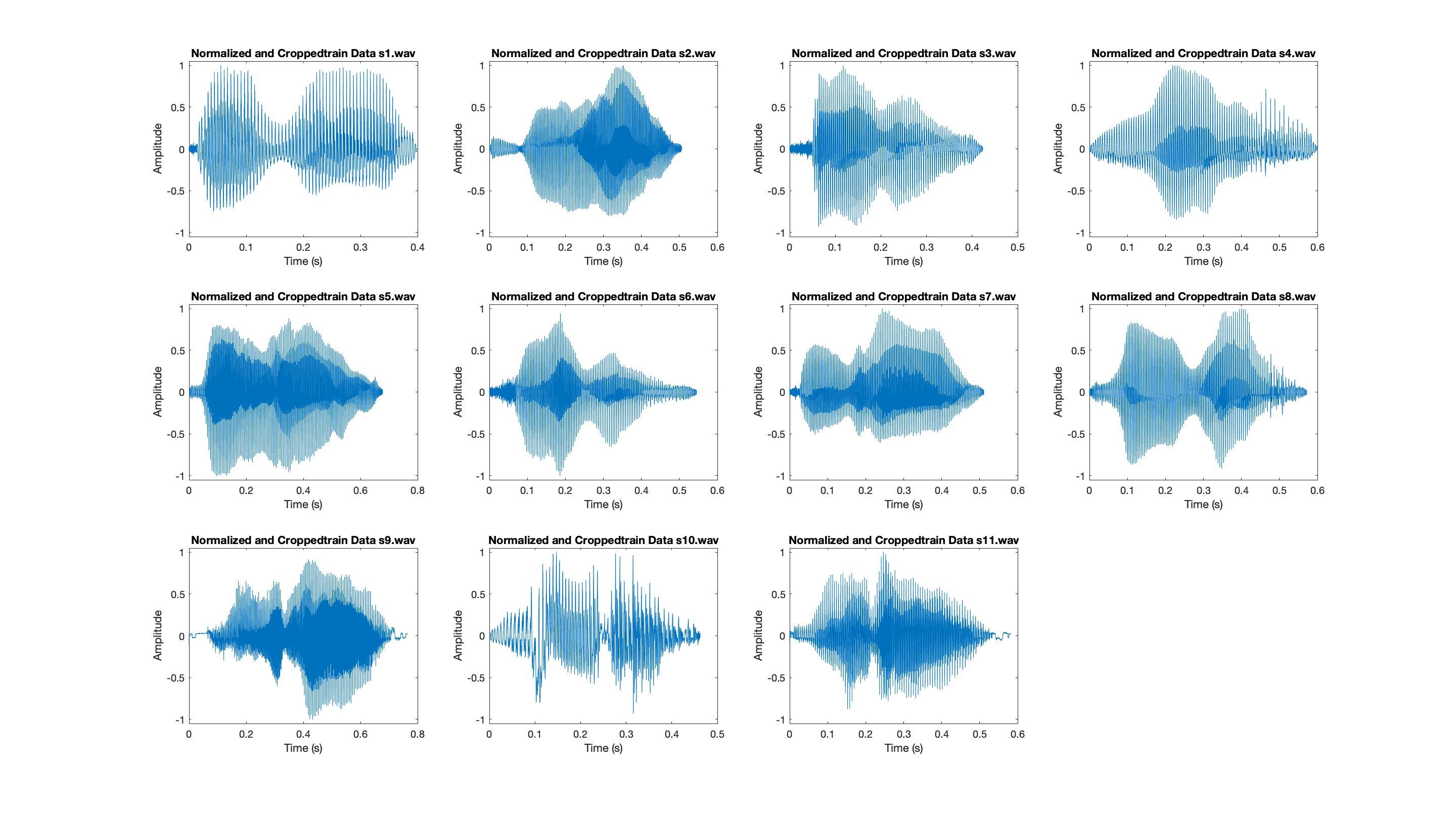 Figure B3: Time domain plots of Processed speechfiles
 Figure B4: Spectrograms of Processed speechfiles
Studies have shown that humans perceive the frequency contents of sounds in a non-linear scale. Each tone with an actual frequency f (Hz) have a corresponding subjective pitch in a scale called 'mel' scale. The mel-frequency scale has linear spacing below 1kHz and logarithmic spacing above 1kHz. One can simulate the mel-frequency scale by generating a filter bank spaced uniformly on the mel-scale. We use a total of 20 filters in this project and the plot of used mel-spaced filter bank response is shown in Figure B5. This filter bank response is generated using 'melfb.m'.

Figure B5: Mel-Spaced Filter Bank Response with 20 coefficients
After applying the Mel-spaced filter bank response to our processed speeechfile spectrum, we get the Mel-Spectrum shown in Figure B6. We see that applying mel-spaced filterbank made the low-frequency components stand out more.

Figure B6: Mel-Spectrum
Finally, we compute the cepstrum and convert log mel spectrum back to time. We apply discrete-cosine transform (DCT) to log mel spectrum and obtain mel frequency cepstrum coefficients (MFCC). MFCCs are the features of our speaker identification algorithm. We normalized the MFCC to make them in range [-1 1] and avoid sparsity of our features. We plot the normalized MFCC of 11 speechfiles in Figure B7. The 0 coefficient is ignored since it represents the mean of the continuous time audio data and is irrelevant in speaker identification.
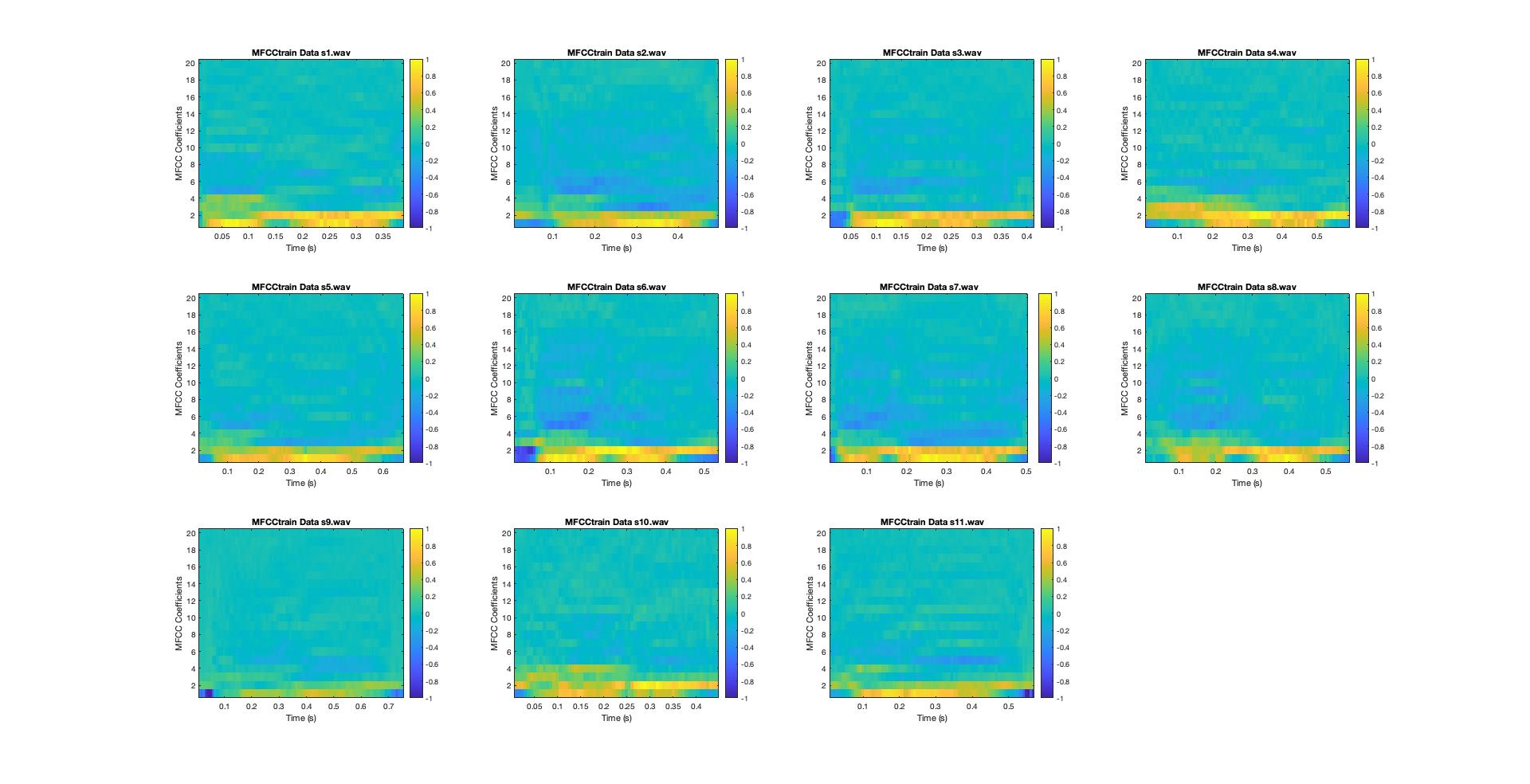
Figure B7: Normalized Mel Frequency Cepstrum Coefficients (MFCC)
In this project we use Vector Quantization (VQ) as the basis of our speaker identifier. VQ maps vectors from a large vector space to a few clusters represented by a codeword. Codeword is the center of a cluster. The collection of all codewords is a codebook. We create a codebook for each speaker using our train data and use it as a reference to identify speakers in the test data. In order to create clusters and find their centroids we use the LBG algorithm following the flow-chart shown in Figure C0. The code is under 'LBG.m'.

Figure C0: Flow diagram of LBG algorithm (Adopted from Rabiner and Juang, 1993)
Figure C1 shows the 2-D vector MFCC space for speakers 3 and 10. MFCC 2 and 3 are used for this 2-D space. We show the codewords (centroids) for 4 clusters. We see that in 2-D MFCC space speakers 3 and 10 form separate clusters and this shows that using the codebook as a reference to identify speakers is a promising method. The VQ-distortion is the metric we use to compare the test data to our reference/codebook. Figure C2 shows all 11 speakers in 2D MFCC space with their respective codewords when clustered into 4 clusters. 'VQ.m' can be executed to obtain the plots in figures C1 and C2.

Figure C1: MFCC Space and Codewords for 4-clusters

Figure C2: MFCC Space and Codewords for 4-clusters
Now that our codebooks are ready we are ready to start identifying speakers. As mentioned in the previous section we compute the VQ-distortion between audio files in test data and the codebooks generated from training data. Figiure D0 shows an overview of the classification. The reference is our codebooks. We use 20 filters in mel-spaced filter bank, 20 MFCC features and 16 clusters to generate our codebooks and obtain the results presented later in this section. There are several tests we performed to test the robustness of our system. The speaker identifier function is under 'classify.m'. We created ground truth table to compute the accuracy of our model.

Figure D0: Basic structure of speaker identification system
We first start by creating a codebook from the training data when all 11 speakers are present in the training data. Therefore, there are no unknown speakers in the test data. This way our model gave us an accuracy of 100% on training data and 81.82% accuracy on testing data. The human performance accuracy is recorded as 62.5% (average between two human performances) on 11 speechfiles. Therefore, our model performs better than human benchmark.
We next include only 8 speakers in training data and test on 11 speakers. Therefore, there are 3 unknown speakers in the test data. In order to reject the unknown speakers and classify them as unknown, we set a threshold of 0.15 to VQ-distortion. Meaning that if minimum VQ-distortion is greater than 0.15 we reject the speaker. 2 out of 3 speakers were correctly classified as unknown. We got an accuracy of 71.73% on test data.
We proceeded to adding new speechfiles to our dataset. We collected speech from three different people and separate recordings for training and testing. We then trained on a total of 14 speechfiles and tested on 14 speechfiles. This was an important step to test our model because the original dataset with 11 audiofiles used the same files for training and testing but now we added 3 audiofiles that have separate training and testing recordings. We achieved an accuracy of 71.43% on this new test data.
To replicate these results run 'classifying_voices.mlx'.
A notch filter/band-stop filter prevents a specific range of frequencies from passing through. In speech recognition, it can be used to drop a particular frequency range from the speech signal. Usually, human speech consists of frequencies of around 100-300Hz. To determine the robustness of our speech recognition system, we chopped-off different frequency intervals from the speech signals and recorded its effect on the system accuracy. We started off by taking even intervals along the entire frequency range. Afterwards, we tried leaving off adult male and female voice ranges as well.
When cropping off lower frequencies, (0 - 1250Hz), the system got only a single testing example correct. For the rest of the testing samples, the Euclidean distance from the training centroids were extremely high and subsequently they were detected as an unknown speaker. The results are slightly better when we cropped off a slightly higher range (1250 – 2500 Hz). Although its not as good as the original test set. But using a notch filter with any interval starting off at higher than 2500 Hz gave the same results as using the entire frequency range. Adult female vocal frequencies range from 165Hz to 255Hz. When we cropped off this portion of the audio, the estimation accuracy drastically fell for female speakers in the test set (Speaker 1 – 9). The system was only able to correctly detect two speakers in this case while the rest were detected as unknown. Strangely, when dropping the adult male frequency range (85-180 Hz), we expected the system to not be able to detect any of the male speakers in the test set. Since, this range is disjoint from the adult female vocal frequency range, we also expected the system to have similar accuracy to using the entire frequency range for female speakers. While the later assumption is somewhat true with only an exception in a single case, the first assumption was not true. The detection system was able to correctly guess both the male speakers from the test set.

Figure D1: Results with Different Notch Filters
The Dataset used for training can be found at https://github.com/Jakobovski/free-spoken-digit-dataset This dataset contains 50 voice samples of different speakers
We trained two seperate systems using the online dataset. First we tried training with only the online dataset by separating a single sample from each speaker and setting that as the training sample and keeping the rest of them for testing. Afterwards, we merged the training samples provided in Canvas with these online training samples while still keeping the testing sample the same.
Using only the online training dataset, our training accuracy was 100% and testing accuracy on 49 x 6 = 294 samples was 75.17%
The confusion matrix for the training case is given below wehere each row corresponds to the ground-truth speaker and the columns correspond to the speaker estimate generated by the system. Additionally, the 7th column corresponds to detecting an unknown speaker.

Using a combined training dataset, the training accuracy still remained at a 100% but for this case the testing accuracy, using the same online dataset as the previous case, dropped significantly to 39.46%.
The confusion matrix for this case is given below where each row corresponds to the ground truth and the each column corresponds to the speaker estiamte generated by the system. Here, speakers 1 - 6 come from the online dataset while speakers 7 - 17 are from the canvas dataset provided to us. The 18th column corresponds to detecting an unknown speaker.
