Home
Grafici GFX is a data plotting library for Adafruit GFX graphic libraries. This modular library allows you to easily manage and plot data on any arduino display/lcd supporting the Adafruit GFX library.
Download the Grafici library via Arduino IDE. This should download also the Adafruit_GFX library.
-
Sketch>Include Library>Manage Libraries(SHIFT + CMD + I) - Search for
Grafici - Select
Grafici-GFXand clickInstall,Install all
Open the simple plot example
-
File>Examples>Grafici-GFX>line_from_array
If you are not using a standard Adafruit TFT shield, change the lines below to match your configuration
#include Adafruit_ILI9341.h
Adafruit_ILI9341 tft = Adafruit_ILI9341(10, 9);
Compile and upload the code to your Arduino
-
Edit>Upload(CMD + U)
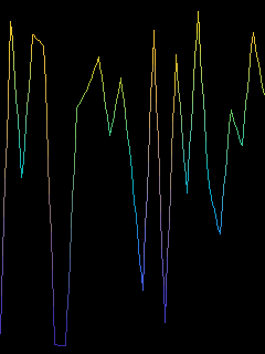
The Arduino's display should show the following
There is no formula to use to plot the Gartner hype cycle. This is because it is a graphical presentation for the maturity, adoption, and social application of specific technologies.
Let start with the initial hype for a technology ( hype = 0 ). After a Technology Trigger the hype reach its Peak of Inflated Expectations ( hype = 100 ). After, interest in the technology wanes as experiments and implementations fail to deliver. This is known as the Trough of Disillusionment ( hype = 20 ). After this pessimistic period, more instances of how the technology can benefit the enterprise start to crystallize and become more widely understood. This is called the Slope of Enlightenment ( hype = 50 ), a growth that only stabilize when mainstream adoption starts to take off. This final phase is called Plateau of Productivity ( hype = 60 ).
To draw the Gartner hype cycle we will declare a representign the various phases of the cycle and then we will interpolate these data points.
unsigned int hype_raw[] = {0, 100, 20, 50, 60, 60, 60};We can now create the hype DataSource from the hype_raw c array (7 elements)
DataArrayXY<int> hype{ hype_raw, 7 };and the interpolated DataSource interpolated_hype_cycle (30 elements) from the DataSource hype.
DataSpline<30> interpolated_hype_cycle{hype.x(),hype.y()};Now we just need to plot interpolated_hype_cycle
plot.line(interpolated_hype_cycle.x(), interpolated_hype_cycle.y(), interpolated_hype_cycle.y());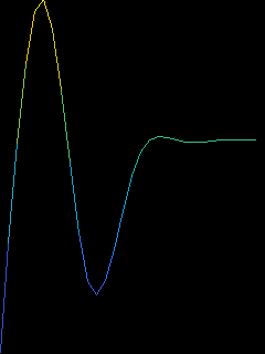
The Grafici library work following few concepts. The easiest way to explain them is to start from the main drawing functions
Grafici plot{ gfx };
plot.line(x, y, color, full_screen);
In these two lines of code we have all the main elements of the Grafici library
- The
Graficiobject plot - Three
DataSourceNormobjects x, y, and color - A
Windowobject full_screen
The Grafici class represents the main interface of the library to the user. There is only one constructor for this class
public inline Grafici (Adafruit_GFX & gfx)where gfx is a display driver implementing the well knwon Adafruit_GFX interface (for Arduino®). If there is no available display driver for your specific use, it is possible to create your own driver with minimal effort. As an example, File_GFX.h is a simple display driver for the Grafici's unit test suite that dumps the display pixels to a bitmap file.
A DataSourceNorm class represent a source of data for plotting. This family of classes behave like a minimal std::vector<DataNorm>. In particular:
- The size of
DataSourceNormcan be queried viaDataSourceNorm::size() - The elements of a
DataSourceNormcan be obtained with the[]operator - The data type returned by
DataSourceNormisDataNorm, a class representing a normalized number, i.e. a floating point between 0.0 and 1.0
NOTE: Internally, the Grafici library handles all data as normalized numbers. It is possible to access the original value of a normalize number via
DataNorm::raw()
As an example, we can create a DataSourceNorm class from an array with the (templated) class DataArray
int src_array[5] = { -10, -5, 0, 5, 10 };
DataArray<int> datasource(src_array, 5);
and access the DataNorm objects with the [] operator. Then the raw and normalized data can be obtained with DataNorm::raw() and DataNorm::norm() methods, repectively.
for(int i = 0; i < 5; ++i)
{
    printf("data[%d] -> raw: %2.2f, norm: %2.2f\n", i, datasource[i].raw(), datasource[i].norm());
}
Will output
data[0] -> raw: -10.00, norm: 0.00
data[1] -> raw:  -5.00, norm: 0.25
data[2] -> raw:   0.00, norm: 0.50
data[3] -> raw:   5.00, norm: 0.75
data[4] -> raw:  10.00, norm: 1.00
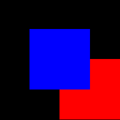
A Window class represent an area of the display in normalized coordinates. The main goal of the Window class is to to draw to a sub-region of the screen withouth worring about the absolute coordinates. As an example,
Window display_window{ { .5, 1 }, {0, .5 } };declares a window occupying a quarter of the screen from 0.5 * width to 1 * width and from 0 * height to 0.5 * height, i.e. the right-bottom quarter.
Drawing a red rectangle from 0,0 (bottom left) to 1,1 (top right) will result in filling the whole region represented by display_window. This is because the coordinates are noormalized and relative to the parent Window.
NOTE: to simplify things, the example skips the plotting layer and call directly the display driver functions
display_driver.fill_rect({ 0, 0 }, { 1, 1 }, red, display_window);
We can draw another rectangle, from 0.25,0.25 to 0.75,0.75. If we draw it against display_window, the drawing coordinates will be relative to the region represented by the Window.
display_driver.fill_rect({ .25, .25 }, { .75, .75 }, blue, display_window);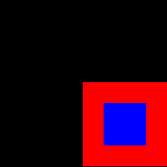
If we instead draw the same blue rectangle against full_screen, an inplicitly declared Window representing the whole display, the rectangle coordinates will be relative to the full screen.
display_driver.fill_rect({ .25, .25 }, { .75, .75 }, blue, full_screen);