Estimate the IMF for an observed cluster, given estimates of its individual masses.
Install the requirements in a conda environment with:
$ conda create --name imfenv python=3.11 numpy matplotlib astropy
$ conda activate imfenv
Binning can create biases when estimating the IMF Apellániz & Úbeda (2005).
The method employed here was originally developed in Khalaj & Baumgardt (2013) and used in Sheikhi et al. (2016). It bypasses the need to bin the masses.
This method diverges for alpha=1, which means it can not fit this IMF slope value.
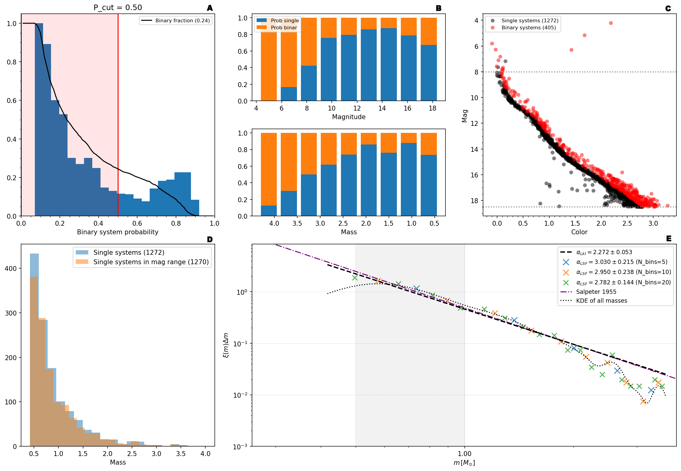
The plots in the output figure represent the following analysis:
A.
The histogram shows the distribution of binary probabilities (BPs) estimated by
ASteCA. This is the probability that a given star in the CMD is a binary
system. Hence: a low BP value means that the star is most likely a single
system, and a large BP means it is most likely a binary system.
The region shaded light red shows the BPs of the stars that were selected for
the subsequent analysis. This selection is performed by fixing the binar_cut
parameter, which represent the probability value that separates single stars
from binary systems. Stars with BPs below this value will be considered
single stars, and binary systems for stars above this value.
The black curve shows the binary fraction of the cluster for different values
of the binar_cut parameter. It has a value of 1 for binar_cut=0 (since all
stars are considered to be binaries) and 0 for binar_cut=1 (since now all
stars are considered to be single systems)
B. Shows the probability of a star in a given magnitude range (top plot) or mass range (bottom plot) of being either a binary system (orange bar), or a single system (blue bar). Notice that both bars add up to 1 since the probability of being a binary is 1 minus the probability of being a single system (no systems of higher number are considered, i.e. ternary, etc.)
C. CMD of the input data. The stars colored in black are those that are used in the analysis, selected as described in plot A. The rest (red stars) are ignored.
The user can also restrict the analysis to a magnitude range using the parameters:
mag_min        = 4
mag_max        = 25
D. Histogram of all single systems' masses and of the selected single systems' masses.
E. The dashed black line shows the maximum likelihood fit (as described in Khalaj & Baumgardt 2013) on the selected set of stars shown in plot C as black points. The Salpeter (1955) slope is also shown, for comparison.
The colored crosses show the slope values that one would obtain applying the
simpler histogram fit on the selected set of stars, for three different number
of bins used, where LSF stands for Least Squares Fit.
The gray shaded region below m=1 shows the region where most of the
theoretical IMFs split their functions. The brown dotted line is the KDE of all
the observed stars, for comparison.
Related literature:
- CCD photometric and mass function study of nine young Large Magellanic Cloud star clusters, Kumar et al. (2008)
- On the function describing the stellar initial mass function, Maschberger (2012)
- Mass distribution and structural parameters of Small Magellanic Cloud star clusters, Maia et al. (2013).
- The Range of Variation of the Mass of the Most Massive Star in Stellar Clusters Derived from 35 Million Monte Carlo Simulations, Popescu & Hanson (2014)