06 May 22:02

Release 0.36.0

New features since last release

Estimate errors in a quantum circuit 🧮

This version of PennyLane lays the foundation for estimating the total error in a quantum circuit from the combination of individual gate errors. (#5154) (#5464) (#5465) (#5278) (#5384)

Two new user-facing classes enable calculating and propagating gate errors in PennyLane:

qml.resource.SpectralNormError: the spectral norm error is defined as the distance, in spectral norm, between the true unitary we intend to apply and the approximate unitary that is actually applied.
qml.resource.ErrorOperation: a base class that inherits from qml.operation.Operation and represents quantum operations which carry some form of algorithmic error.

SpectralNormError can be used for back-of-the-envelope type calculations like obtaining the spectral norm error between two unitaries via get_error:
```
import pennylane as qml 
from pennylane.resource import ErrorOperation, SpectralNormError

intended_op = qml.RY(0.40, 0) 
actual_op = qml.RY(0.41, 0) # angle of rotation is slightly off
```
```
>>> SpectralNormError.get_error(intended_op, actual_op) 
0.004999994791668309 
```
SpectralNormError is also a key tool to specify errors in larger quantum circuits:
For operations representing a major building block of an algorithm, we can create a custom operation that inherits from ErrorOperation. This child class must override the error method and should return a SpectralNormError instance:
```
class MyErrorOperation(ErrorOperation):
   
   def __init__(self, error_val, wires): 
       self.error_val = error_val 
       super().__init__(wires=wires)

   def error(self): 
       return SpectralNormError(self.error_val)
```
In this toy example, MyErrorOperation introduces an arbitrary SpectralNormError when called in a QNode. It does not require a decomposition or matrix representation when used with null.qubit (suggested for use with resource and error estimation since circuit executions are not required to calculate resources or errors).
```
dev = qml.device("null.qubit")

@qml.qnode(dev) 
def circuit(): 
   MyErrorOperation(0.1, wires=0) 
   MyErrorOperation(0.2, wires=1) 
   return qml.state() 
```
The total spectral norm error of the circuit can be calculated using qml.specs:
```
>>> qml.specs(circuit)()['errors'] 
{'SpectralNormError': SpectralNormError(0.30000000000000004)} 
```
PennyLane already includes a number of built-in building blocks for algorithms like QuantumPhaseEstimation and TrotterProduct. TrotterProduct now propagates errors based on the number of steps performed in the Trotter product. QuantumPhaseEstimation now propagates errors based on the error of its input unitary.
```
dev = qml.device('null.qubit') 
hamiltonian = qml.dot([1.0, 0.5, -0.25], [qml.X(0), qml.Y(0), qml.Z(0)])

@qml.qnode(dev) 
def circuit(): 
   qml.TrotterProduct(hamiltonian, time=0.1, order=2) 
   qml.QuantumPhaseEstimation(MyErrorOperation(0.01, wires=0), estimation_wires=[1, 2, 3]) 
   return qml.state()
```
Again, the total spectral norm error of the circuit can be calculated using qml.specs:
```
>>> qml.specs(circuit)()["errors"] 
{'SpectralNormError': SpectralNormError(0.07616666666666666)} 
```
Check out our error propagation demo to see how to use these new features in a real-world example!

Access an extended arsenal of quantum algorithms 🏹

The Fast Approximate BLock-Encodings (FABLE) algorithm for embedding a matrix into a quantum circuit as outlined in arXiv:2205.00081 is now accessible via the qml.FABLE template. (#5107)

The usage of qml.FABLE is similar to qml.BlockEncode but provides a more efficient circuit construction at the cost of a user-defined approximation level, tol. The number of wires that qml.FABLE operates on is 2*n + 1, where n defines the dimension of the $2^n \times 2^n$ matrix that we want to block-encode.
```
import numpy as np

A = np.array([[0.1, 0.2], [0.3, 0.4]]) 
dev = qml.device('default.qubit', wires=3)

@qml.qnode(dev) 
def circuit(): 
   qml.FABLE(A, tol = 0.001, wires=range(3)) 
   return qml.state() 
```
```
>>> mat = qml.matrix(circuit)() 
>>> 2 * mat[0:2, 0:2] 
array([[0.1+0.j, 0.2+0.j], [0.3+0.j, 0.4+0.j]]) 
```
A high-level interface for amplitude amplification and its variants is now available via the new qml.AmplitudeAmplification template. (#5160)

Based on arXiv:quant-ph/0005055, given a state $\vert \Psi \rangle = \alpha \vert \phi \rangle + \beta \vert \phi^{\perp} \rangle$, qml.AmplitudeAmplification amplifies the amplitude of $\vert \phi \rangle$.

Here's an example with a target state $\vert \phi \rangle = \vert 2 \rangle = \vert 010 \rangle$, an input state $\vert \Psi \rangle = H^{\otimes 3} \vert 000 \rangle$, as well as an oracle that flips the sign of $\vert \phi \rangle$ and does nothing to $\vert \phi^{\perp} \rangle$, which can be achieved in this case through qml.FlipSign.
```
@qml.prod 
def generator(wires): 
   for wire in wires: 
       qml.Hadamard(wires=wire)

U = generator(wires=range(3)) 
O = qml.FlipSign(2, wires=range(3)) 
```
Here, U is a quantum operation that is created by decorating a quantum function with @qml.prod. This could alternatively be done by creating a user-defined custom operation with a decomposition. Amplitude amplification can then be set up within a circuit:
```
dev = qml.device("default.qubit")

@qml.qnode(dev) 
def circuit(): 
   generator(wires=range(3)) # prepares |Psi> = U|0> 
   qml.AmplitudeAmplification(U, O, iters=10)
   return qml.probs(wires=range(3)) 
```
```
>>> print(np.round(circuit(), 3)) 
[0.01 0.01 0.931 0.01 0.01 0.01 0.01 0.01 ] 
```
As expected, we amplify the $\vert 2 \rangle$ state.
Reflecting about a given quantum state is now available via qml.Reflection. This operation is very useful in the amplitude amplification algorithm and offers a generalization of qml.FlipSign, which operates on basis states. (#5159)

qml.Reflection works by providing an operation, $U$, that prepares the desired state, $\vert \psi \rangle$, that we want to reflect about. In other words, $U$ is such that $U \vert 0 \rangle = \vert \psi \rangle$. In PennyLane, $U$ must be an Operator. For example, if we want to reflect about $\vert \psi \rangle = \vert + \rangle$, then $U = H$:
```
U = qml.Hadamard(wires=0)
dev = qml.device('default.qubit') 

@qml.qnode(dev) 
def circuit(): 
   qml.Reflection(U) 
   return qml.state() 
```
```
>>> circuit() 
tensor([0.-6.123234e-17j, 1.+6.123234e-17j], requires_grad=True) 
```

Performing qubitization is now easily accessible with the new qml.Qubitization operator. (#5500)

qml.Qubitization encodes a Hamiltonian into a suitable unitary operator. When applied in conjunction with quantum phase estimation (QPE), it allows for computing the eigenvalue of an eigenvector of the given Hamiltonian.

H = qml.dot([0.1, 0.3, -0.3], [qml.Z(0), qml.Z(1), qml.Z(0) @ qml.Z(2)]) 
@qml.qnode(qml.device("default.qubit")) 
def circuit(): 
   # initialize the eigenvector 
   qml.PauliX(2) 
   # apply QPE 
   measurements = qml.iterative_qpe(
       qml.Qubitization(H, control = [3,4]), ancilla = 5, iters = 3
   ) 
   return qml.probs(op = measurements)

Make use of more methods to map from molecules 🗺️

A new function called qml.bravyi_kitaev has been added to perform the Bravyi-Kitaev mapping of fermionic Hamiltonians to qubit Hamiltonians. (#5390)

This function presents an alternative mapping to qml.jordan_wigner or qml.parity_transform which can help us measure expectation values more efficiently on hardware. Simply provide a fermionic Hamiltonian (created from from_string, FermiA, FermiC, FermiSentence, or FermiWord) and the number of qubits / spin orbitals in the system, n:
```
>>> fermi_ham = qml.fermi.from_string('0+ 1+ 1- 0-') 
>>> qubit_ham = qml.bravyi_kitaev(fermi_ham, n=6, tol=0.0) 
>>> print(qubit_ham) 
0.25 * I(0) + -0.25 * Z(0) + -0.25 * (Z(0) @ Z(1)) + 0.25 * Z(1) 
```
The qml.qchem.hf_state function has been upgraded to be compatible with qml.parity_transform and the new Bravyi-Kitaev mapping (qml.bravyi_kitaev). (#5472) (#5472)
```
>>> state_bk = qml.qchem.hf_state(2, 6, basis="bravyi_kitaev") 
>>> print(state_bk) 
[1 0 0 ...
```

Assets 2

11 Mar 21:09

Mandrenkov

v0.35.1

db2fb6d

Release 0.35.1

Bug fixes 🐛

Lightning simulators need special handling of diagonalizing gates when performing sampling measurements. (#5343)
Updated the lower bound on the required Catalyst version to v0.5.0. (#5320)

Contributors ✍️

This release contains contributions from (in alphabetical order):

Vincent Michaud-Rioux, Erick Ochoa Lopez.

Assets 2

04 Mar 20:25

lillian542

v0.35.0

cf042f6

Release 0.35.0

New features since last release

Qiskit 1.0 integration 🔌

This version of PennyLane makes it easier to import circuits from Qiskit. (#5218) (#5168)

The qml.from_qiskit function converts a Qiskit QuantumCircuit into a PennyLane quantum function. Although qml.from_qiskit already exists in PennyLane, we have made a number of improvements to make importing from Qiskit easier. And yes — qml.from_qiskit functionality is compatible with both Qiskit 1.0 and earlier versions! Here's a comprehensive list of the improvements:

You can now append PennyLane measurements onto the quantum function returned by qml.from_qiskit. Consider this simple Qiskit circuit:

import pennylane as qml 
from qiskit import QuantumCircuit

qc = QuantumCircuit(2) 
qc.rx(0.785, 0) 
qc.ry(1.57, 1)

We can convert it into a PennyLane QNode in just a few lines, with PennyLane measurements easily included:

>>> dev = qml.device("default.qubit") 
>>> measurements = qml.expval(qml.Z(0) @ qml.Z(1)) 
>>> qfunc = qml.from_qiskit(qc, measurements=measurements) 
>>> qnode = qml.QNode(qfunc, dev) 
>>> qnode() 
tensor(0.00056331, requires_grad=True)

Quantum circuits that already contain Qiskit-side measurements can be faithfully converted with qml.from_qiskit. Consider this example Qiskit circuit:

qc = QuantumCircuit(3, 2) # Teleportation

qc.rx(0.9, 0) # Prepare input state on qubit 0

qc.h(1) # Prepare Bell state on qubits 1 and 2 qc.cx(1, 2)

qc.cx(0, 1) # Perform teleportation 
qc.h(0) 
qc.measure(0, 0) 
qc.measure(1, 1)

with qc.if_test((1, 1)): # Perform first conditional 
    qc.x(2)

This circuit can be converted into PennyLane with the Qiskit measurements still accessible. For example, we can use those results as inputs to a mid-circuit measurement in PennyLane:

@qml.qnode(dev) 
def teleport(): 
    m0, m1 = qml.from_qiskit(qc)() 
    qml.cond(m0, qml.Z)(2) 
    return qml.density_matrix(2)

>>> teleport() 
tensor([[0.81080498+0.j , 0. +0.39166345j], 
[0. -0.39166345j, 0.18919502+0.j ]], requires_grad=True)

It is now more intuitive to handle and differentiate parametrized Qiskit circuits. Consider the following circuit:

from qiskit.circuit import Parameter 
from pennylane import numpy as np

angle0 = Parameter("x") angle1 = Parameter("y")

qc = QuantumCircuit(2, 2) 
qc.rx(angle0, 0) 
qc.ry(angle1, 1) 
qc.cx(1, 0)

We can convert this circuit into a QNode with two arguments, corresponding to x and y:

measurements = qml.expval(qml.PauliZ(0)) 
qfunc = qml.from_qiskit(qc, measurements) 
qnode = qml.QNode(qfunc, dev)

The QNode can be evaluated and differentiated:

>>> x, y = np.array([0.4, 0.5], requires_grad=True) 
>>> qnode(x, y) 
tensor(0.80830707, requires_grad=True) 

>>> qml.grad(qnode)(x, y) 
(tensor(-0.34174675, requires_grad=True), tensor(-0.44158016, requires_grad=True))

This shows how easy it is to make a Qiskit circuit differentiable with PennyLane.

In addition to circuits, it is also possible to convert operators from Qiskit to PennyLane with a new function called qml.from_qiskit_op. (#5251)

A Qiskit SparsePauliOp can be converted to a PennyLane operator using qml.from_qiskit_op:

>>> from qiskit.quantum_info import SparsePauliOp 
>>> qiskit_op = SparsePauliOp(["II", "XY"]) 
>>> qiskit_op SparsePauliOp(['II', 'XY'], coeffs=[1.+0.j, 1.+0.j]) 
>>> pl_op = qml.from_qiskit_op(qiskit_op) 
>>> pl_op I(0) + X(1) @ Y(0)

Combined with qml.from_qiskit, it becomes easy to quickly calculate quantities like expectation values by converting the whole workflow to PennyLane:

qc = QuantumCircuit(2) # Create circuit 
qc.rx(0.785, 0) 
qc.ry(1.57, 1)

measurements = qml.expval(pl_op) # Create QNode 
qfunc = qml.from_qiskit(qc, measurements) 
qnode = qml.QNode(qfunc, dev)

>>> qnode() # Evaluate! 
tensor(0.29317504, requires_grad=True)

Native mid-circuit measurements on Default Qubit 💡

Mid-circuit measurements can now be more scalable and efficient in finite-shots mode with default.qubit by simulating them in a similar way to what happens on quantum hardware. (#5088) (#5120)

Previously, mid-circuit measurements (MCMs) would be automatically replaced with an additional qubit using the @qml.defer_measurements transform. The circuit below would have required thousands of qubits to simulate.

Now, MCMs are performed in a similar way to quantum hardware with finite shots on default.qubit. For each shot and each time an MCM is encountered, the device evaluates the probability of projecting onto |0> or |1> and makes a random choice to collapse the circuit state. This approach works well when there are a lot of MCMs and the number of shots is not too high.
```
import pennylane as qml

dev = qml.device("default.qubit", shots=10)

@qml.qnode(dev) 
def f(): 
    for i in range(1967): 
        qml.Hadamard(0) 
        qml.measure(0) 
    return qml.sample(qml.PauliX(0)) 
```
```
>>> f() 
tensor([-1, -1, -1, 1, 1, -1, 1, -1, 1, -1], requires_grad=True) 
```

Work easily and efficiently with operators 🔧

Over the past few releases, PennyLane's approach to operator arithmetic has been in the process of being overhauled. We have a few objectives:
1. To make it as easy to work with PennyLane operators as it would be with pen and paper.
2. To improve the efficiency of operator arithmetic.
The updated operator arithmetic functionality is still being finalized, but can be activated using qml.operation.enable_new_opmath(). In the next release, the new behaviour will become the default, so we recommend enabling now to become familiar with the new system!

The following updates have been made in this version of PennyLane:
- You can now easily access Pauli operators via I, X, Y, and Z: (#5116)
```
>>> from pennylane import I, X, Y, Z 
>>> X(0) X(0) ```

The original long-form names `Identity`, `PauliX`, `PauliY`, and `PauliZ` remain available, but use of the short-form names is now recommended.
```
- A new qml.commutator function is now available that allows you to compute commutators between PennyLane operators. (#5051) (#5052) (#5098)
```
>>> qml.commutator(X(0), Y(0)) 
2j * Z(0) 
```
- Operators in PennyLane can have a backend Pauli representation, which can be used to perform faster operator arithmetic. Now, the Pauli representation will be automatically used for calculations when available. (#4989) (#5001) (#5003) (#5017) (#5027)
  
  The Pauli representation can be optionally accessed via op.pauli_rep:
```
>>> qml.operation.enable_new_opmath() 
>>> op = X(0) + Y(0) 
>>> op.pauli_rep 
1.0 * X(0) + 1.0 * Y(0) 
```
- Extensive improvements have been made to the string representations of PennyLane operators, making them shorter and possible to copy-paste as valid PennyLane code. (#5116) (#5138)
```
>>> 0.5 * X(0) 
0.5 * X(0)
>>> 0.5 * (X(0) + Y(1)) 
0.5 * (X(0) + Y(1)) 
```
  Sums with many terms are broken up into multiple lines, but can still be copied back as valid code:
```
>>> 0.5 * (X(0) @ X(1)) + 0.7 * (X(1) @ X(2)) + 0.8 * (X(2) @ X(3)) 
( 
     0.5 * (X(0) @ X(1)) 
     + 0.7 * (X(1) @ X(2)) 
     + 0.8 * (X(2) @ X(3)) 
) 
```
- Linear combinations of operators and operator multiplication via Sum and Prod, respectively, have been updated to reach feature parity with Hamiltonian and Tensor, respectively. This should minimize the effort to port over any existing code. (#5070) (#5132) (#5133)
  
  Updates include support for grouping via the pauli module:
```
>>> obs = [X(0) @ Y(1), Z(0), Y(0) @ Z(1), Y(1)] 
>>> qml.pauli.group_observables(obs) 
[[Y(0) @ Z(1)], [X(0) @ Y(1), Y(1)], [Z(0)]] 
```

New Clifford device 🦾

A new default.clifford device enables efficient simulati...

Assets 3

22 Jan 17:04

albi3ro

v0.34.0.post1

11ca3ee

Release 0.34.0.post1

This postfix release pins additional requirements in doc/requirements.txt for building the website documentation. This allows the website to be rebuilt to show the "Getting involved" section.

Assets 2

08 Jan 20:06

lillian542

v0.34.0

1a315b9

Release 0.34.0

New features since last release

Statistics and drawing for mid-circuit measurements 🎨

It is now possible to return statistics of composite mid-circuit measurements. (#4888)

Mid-circuit measurement results can be composed using basic arithmetic operations and then statistics can be calculated by putting the result within a PennyLane measurement like qml.expval(). For example:

import pennylane as qml

dev = qml.device("default.qubit")

@qml.qnode(dev) 
def circuit(phi, theta): 
    qml.RX(phi, wires=0) 
    m0 = qml.measure(wires=0) 
    qml.RY(theta, wires=1) 
    m1 = qml.measure(wires=1) 
    return qml.expval(~m0 + m1)

print(circuit(1.23, 4.56))

1.2430187928114291

Another option, for ease-of-use when using qml.sample(), qml.probs(), or qml.counts(), is to provide a simple list of mid-circuit measurement results:

dev = qml.device("default.qubit")

@qml.qnode(dev) 
def circuit(phi, theta): 
    qml.RX(phi, wires=0) 
    m0 = qml.measure(wires=0) 
    qml.RY(theta, wires=1) 
    m1 = qml.measure(wires=1) 
    return qml.sample(op=[m0, m1])

print(circuit(1.23, 4.56, shots=5))

[[0 1] 
 [0 1] 
 [0 0] 
 [1 0] 
 [0 1]]

Composite mid-circuit measurement statistics are supported on default.qubit and default.mixed. To learn more about which measurements and arithmetic operators are supported, refer to the measurements page and the documentation for qml.measure.

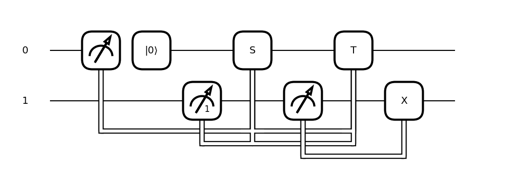
Mid-circuit measurements can now be visualized with the text-based qml.draw() and the graphical qml.draw_mpl() methods. (#4775) (#4803) (#4832) (#4901) (#4850) (#4917) (#4930) (#4957)

Drawing of mid-circuit measurement capabilities including qubit reuse and reset, postselection, conditioning, and collecting statistics is now supported. Here is an all-encompassing example:

def circuit(): 
    m0 = qml.measure(0, reset=True) 
    m1 = qml.measure(1, postselect=1) 
    qml.cond(m0 - m1 == 0, qml.S)(0) 
    m2 = qml.measure(1) 
    qml.cond(m0 + m1 == 2, qml.T)(0) 
    qml.cond(m2, qml.PauliX)(1)

The text-based drawer outputs:

>>> print(qml.draw(circuit)()) 
0: ──┤↗│  │0⟩────────S───────T────┤ 
1: ───║────────┤↗₁├──║──┤↗├──║──X─┤ 
      ╚═════════║════╬═══║═══╣  ║ 
                ╚════╩═══║═══╝  ║ 
                         ╚══════╝

The graphical drawer outputs:

>>> print(qml.draw_mpl(circuit)())

Catalyst is seamlessly integrated with PennyLane ⚗️

Catalyst, our next-generation compilation framework, is now accessible within PennyLane, allowing you to more easily benefit from hybrid just-in-time (JIT) compilation.

To access these features, simply install pennylane-catalyst:
```
pip install pennylane-catalyst 
```
The qml.compiler module provides support for hybrid quantum-classical compilation. (#4692) (#4979)

Through the use of the qml.qjit decorator, entire workflows can be JIT compiled — including both quantum and classical processing — down to a machine binary on first-function execution. Subsequent calls to the compiled function will execute the previously-compiled binary, resulting in significant performance improvements.
```
import pennylane as qml

dev = qml.device("lightning.qubit", wires=2)

@qml.qjit 
@qml.qnode(dev) 
def circuit(theta): 
    qml.Hadamard(wires=0) 
    qml.RX(theta, wires=1) 
    qml.CNOT(wires=[0,1]) 
    return qml.expval(qml.PauliZ(wires=1)) 
```
```
>>> circuit(0.5) # the first call, compilation occurs here array(0.) 
>>> circuit(0.5) # the precompiled quantum function is called 
array(0.) 
```
Currently, PennyLane supports the Catalyst hybrid compiler with the qml.qjit decorator. A significant benefit of Catalyst is the ability to preserve complex control flow around quantum operations — such as if statements and for loops, and including measurement feedback — during compilation, while continuing to support end-to-end autodifferentiation.

The following functions can now be used with the qml.qjit decorator: qml.grad, qml.jacobian, qml.vjp, qml.jvp, and qml.adjoint. (#4709) (#4724) (#4725) (#4726)

When qml.grad or qml.jacobian are used with @qml.qjit, they are patched to catalyst.grad and catalyst.jacobian, respectively.

dev = qml.device("lightning.qubit", wires=1)

@qml.qjit 
def workflow(x):

    @qml.qnode(dev) 
    def circuit(x): 
        qml.RX(np.pi * x[0], wires=0) 
        qml.RY(x[1], wires=0) 
        return qml.probs()

    g = qml.jacobian(circuit)

    return g(x)

>>> workflow(np.array([2.0, 1.0])) 
array([[ 3.48786850e-16, -4.20735492e-01], 
       [-8.71967125e-17, 4.20735492e-01]])

JIT-compatible functionality for control flow has been added via qml.for_loop, qml.while_loop, and qml.cond. (#4698)

qml.for_loop and qml.while_loop can be deployed as decorators on functions that are the body of the loop. The arguments to both follow typical conventions:

@qml.for_loop(lower_bound, upper_bound, step)

@qml.while_loop(cond_function)

Here is a concrete example with qml.for_loop:

dev = qml.device("lightning.qubit", wires=1)

@qml.qjit 
@qml.qnode(dev) 
def circuit(n: int, x: float):

    @qml.for_loop(0, n, 1) 
    def loop_rx(i, x): 
        # perform some work and update (some of) the arguments 
        qml.RX(x, wires=0)

        # update the value of x for the next iteration 
        return jnp.sin(x)

    # apply the for loop 
    final_x = loop_rx(x)

    return qml.expval(qml.PauliZ(0)), final_x

>>> circuit(7, 1.6) 
(array(0.97926626), array(0.55395718))

Decompose circuits into the Clifford+T gateset 🧩

The new qml.clifford_t_decomposition() transform provides an approximate breakdown of an input circuit into the Clifford+T gateset. Behind the scenes, this decomposition is enacted via the sk_decomposition() function using the Solovay-Kitaev algorithm. (#4801) (#4802)

The Solovay-Kitaev algorithm approximately decomposes a quantum circuit into the Clifford+T gateset. To account for this, a desired total circuit decomposition error, epsilon, must be specified when using qml.clifford_t_decomposition:

dev = qml.device("default.qubit")

@qml.qnode(dev) 
def circuit(): 
    qml.RX(1.1, 0) 
    return qml.state()

circuit = qml.clifford_t_decomposition(circuit, epsilon=0.1)

>>> print(qml.draw(circuit)()) 
0:   ──T†──H──T†──H──T──H──T──H──T──H──T──H──T†──H──T†──T†──H──T†──H──T──H──T──H──T──H──T──H──T†──H

 ───T†──H──T──H──GlobalPhase(0.39)─┤

The resource requirements of this circuit can also be evaluated:

>>> with qml.Tracker(dev) as tracker: 
...     circuit() 
>>> resources_lst = tracker.history["resources"] 
>>> resources_lst[0] 
wires: 1 
gates: 34 
depth: 34 
shots: Shots(total=None) 
gate_types: {'Adjoint(T)': 8, 'Hadamard': 16, 'T': 9, 'GlobalPhase': 1} 
gate_sizes:   {1: 33, 0: 1}

Use an iterative approach for quantum phase estimation 🔄

Iterative Quantum Phase Estimation is now available with qml.iterative_qpe. (#4804)

The subroutine can be used similarly to mid-circuit measurements:

import pennylane as qml

dev = qml.device("default.qubit", shots=5)

@qml.qnode(dev) 
def circuit():

      # Initial state 
      qml.PauliX(wires=[0])

      # Iterative QPE 
      measurements = qml.iterative_qpe(qml.RZ(2., wires=[0]), ancilla=[1], iters=3)

      return [qml.sample(op=meas) for meas in measurements]

>>> print(circuit()) 
[array([0, 0, 0, 0, 0]), array([1, 0, 0, 0, 0]), array([0, 1, 1, 1...

Assets 2

08 Nov 20:57

timmysilv

v0.33.1

4d9ea4d

Release 0.33.1

Bug fixes 🐛

Fix gradient performance regression due to expansion of VJP products. (#4806)
qml.defer_measurements now correctly transforms circuits when terminal measurements include wires used in mid-circuit measurements. (#4787)
Any ScalarSymbolicOp, like Evolution, now states that it has a matrix if the target is a Hamiltonian. (#4768)
In default.qubit, initial states are now initialized with the simulator's wire order, not the circuit's wire order. (#4781)

Contributors ✍️

This release contains contributions from (in alphabetical order):

Christina Lee, Lee James O'Riordan, Mudit Pandey

Assets 2

30 Oct 20:13

mudit2812

v0.33.0

1b20871

Release 0.33.0

New features since last release

Postselection and statistics in mid-circuit measurements 📌

It is now possible to request postselection on a mid-circuit measurement. (#4604)

This can be achieved by specifying the postselect keyword argument in qml.measure as either 0 or 1, corresponding to the basis states.
```
import pennylane as qml

dev = qml.device("default.qubit")

@qml.qnode(dev, interface=None)
def circuit():
    qml.Hadamard(wires=0)
    qml.CNOT(wires=[0, 1])
    qml.measure(0, postselect=1)
    return qml.expval(qml.PauliZ(1)), qml.sample(wires=1)
```
This circuit prepares the $| \Phi^{+} \rangle$ Bell state and postselects on measuring $|1\rangle$ in wire 0. The output of wire 1 is then also $|1\rangle$ at all times:
```
>>> circuit(shots=10)
(-1.0, array([1, 1, 1, 1, 1, 1]))
```
Note that the number of shots is less than the requested amount because we have thrown away the samples where $|0\rangle$ was measured in wire 0.

Measurement statistics can now be collected for mid-circuit measurements. (#4544)

dev = qml.device("default.qubit")

@qml.qnode(dev)
def circ(x, y):
    qml.RX(x, wires=0)
    qml.RY(y, wires=1)
    m0 = qml.measure(1)
    return qml.expval(qml.PauliZ(0)), qml.expval(m0), qml.sample(m0)

>>> circ(1.0, 2.0, shots=10000)
(0.5606, 0.7089, array([0, 1, 1, ..., 1, 1, 1]))

Support is provided for both finite-shot and analytic modes and devices default to using the deferred measurement principle to enact the mid-circuit measurements.

Exponentiate Hamiltonians with flexible Trotter products 🐖

Higher-order Trotter-Suzuki methods are now easily accessible through a new operation called TrotterProduct. (#4661)

Trotterization techniques are an affective route towards accurate and efficient Hamiltonian simulation. The Suzuki-Trotter product formula allows for the ability to express higher-order approximations to the matrix exponential of a Hamiltonian, and it is now available to use in PennyLane via the TrotterProduct operation. Simply specify the order of the approximation and the evolution time.
```
coeffs = [0.25, 0.75]
ops = [qml.PauliX(0), qml.PauliZ(0)]
H = qml.dot(coeffs, ops)

dev = qml.device("default.qubit", wires=2)

@qml.qnode(dev)
def circuit():
    qml.Hadamard(0)
    qml.TrotterProduct(H, time=2.4, order=2)
    return qml.state()
```
```
>>> circuit()
[-0.13259524+0.59790098j 0. +0.j -0.13259524-0.77932754j 0. +0.j ]
```
Approximating matrix exponentiation with random product formulas, qDrift, is now available with the new QDrift operation. (#4671)

As shown in 1811.08017, qDrift is a Markovian process that can provide a speedup in Hamiltonian simulation. At a high level, qDrift works by randomly sampling from the Hamiltonian terms with a probability that depends on the Hamiltonian coefficients. This method for Hamiltonian simulation is now ready to use in PennyLane with the QDrift operator. Simply specify the evolution time and the number of samples drawn from the Hamiltonian, n:
```
coeffs = [0.25, 0.75]
ops = [qml.PauliX(0), qml.PauliZ(0)]
H = qml.dot(coeffs, ops)

dev = qml.device("default.qubit", wires=2)

@qml.qnode(dev)
def circuit():
    qml.Hadamard(0)
    qml.QDrift(H, time=1.2, n = 10)
    return qml.probs()
```
```
>>> circuit()
array([0.61814334, 0. , 0.38185666, 0. ])
```

Building blocks for quantum phase estimation 🧱

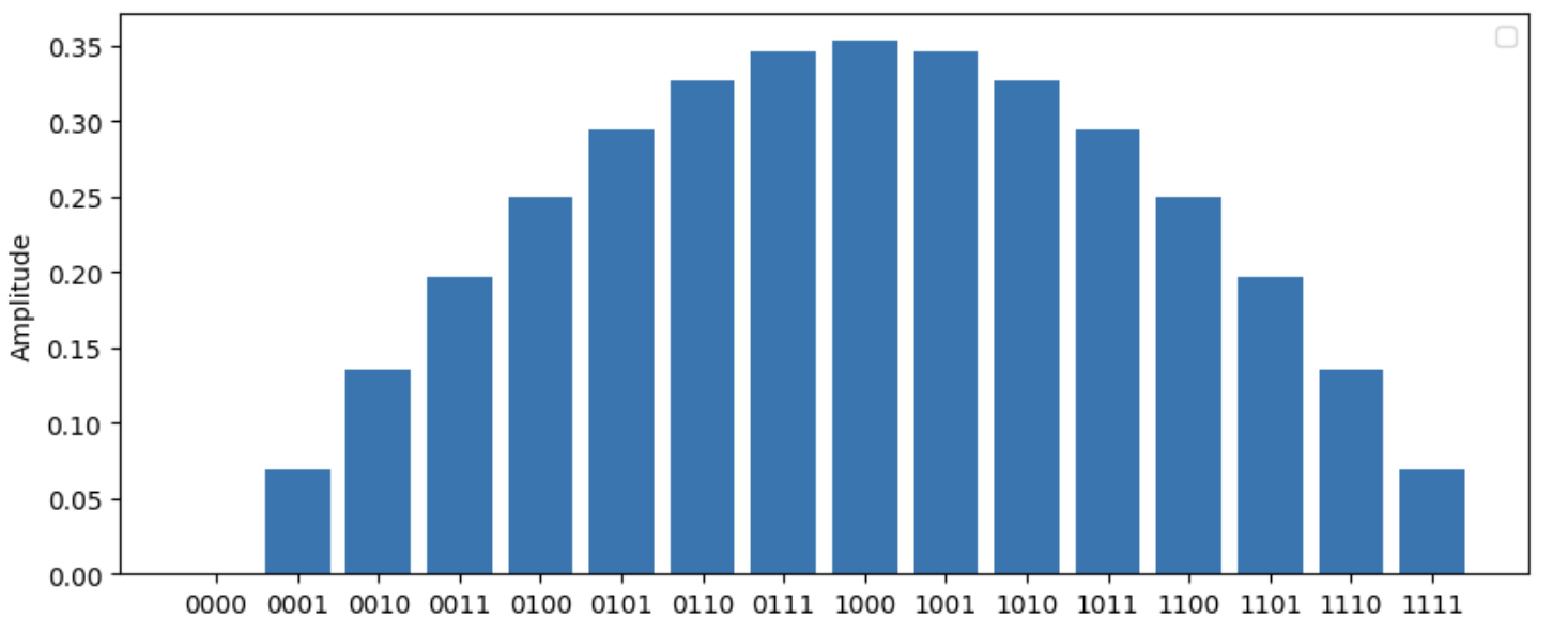
A new operator called CosineWindow has been added to prepare an initial state based on a cosine wave function. (#4683)

As outlined in 2110.09590, the cosine tapering window is part of a modification to quantum phase estimation that can provide a cubic improvement to the algorithm's error rate. Using CosineWindow will prepare a state whose amplitudes follow a cosinusoidal distribution over the computational basis.
```
import matplotlib.pyplot as plt

dev = qml.device('default.qubit', wires=4)

@qml.qnode(dev)
def example_circuit():
    qml.CosineWindow(wires=range(4))
    return qml.state()

output = example_circuit()

plt.style.use("pennylane.drawer.plot")
plt.bar(range(len(output)), output)
plt.show()
```

Controlled gate sequences raised to decreasing powers, a sub-block in quantum phase estimation, can now be created with the new ControlledSequence operator. (#4707)

To use ControlledSequence, specify the controlled unitary operator and the control wires, control:

dev = qml.device("default.qubit", wires = 4)

@qml.qnode(dev)
def circuit():
    for i in range(3):
        qml.Hadamard(wires = i)
    qml.ControlledSequence(qml.RX(0.25, wires = 3), control = [0, 1, 2])
    qml.adjoint(qml.QFT)(wires = range(3))
        return qml.probs(wires = range(3))

>>> print(circuit())
[0.92059345 0.02637178 0.00729619 0.00423258 0.00360545 0.00423258 0.00729619 0.02637178]

New device capabilities, integration with Catalyst, and more! ⚗️

default.qubit now uses the new qml.devices.Device API and functionality in qml.devices.qubit. If you experience any issues with the updated default.qubit, please let us know by posting an issue. The old version of the device is still accessible by the short name default.qubit.legacy, or directly via qml.devices.DefaultQubitLegacy. (#4594) (#4436) (#4620) (#4632)

This changeover has a number of benefits for default.qubit, including:
- The number of wires is now optional — simply having qml.device("default.qubit") is valid! If wires are not provided at instantiation, the device automatically infers the required number of wires for each circuit provided for execution.
```
dev = qml.device("default.qubit")

@qml.qnode(dev)
def circuit():
    qml.PauliZ(0)
    qml.RZ(0.1, wires=1)
    qml.Hadamard(2)
    return qml.state()
```
```
>>> print(qml.draw(circuit)())
0: ──Z────────┤ State
1: ──RZ(0.10)─┤ State
2: ──H────────┤ State
```
- default.qubit is no longer silently swapped out with an interface-appropriate device when the backpropagation differentiation method is used. For example, consider:
```
import jax

dev = qml.device("default.qubit", wires=1)

@qml.qnode(dev, diff_method="backprop")
def f(x):
    qml.RX(x, wires=0)
    return qml.expval(qml.PauliZ(0))
f(jax.numpy.array(0.2))
```
  In previous versions of PennyLane, the device will be swapped for the JAX equivalent:
```
>>> f.device
<DefaultQubitJax device (wires=1, shots=None) at 0x7f8c8bff50a0>
>>> f.device == dev
False
```
  Now, default.qubit can itself dispatch to all the interfaces in a backprop-compatible way and hence does not need to be swapped:
```
>>> f.device
<default.qubit device (wires=1) at 0x7f20d043b040>
>>> f.device == dev
True
```

A QNode that has been decorated with qjit from PennyLane's Catalyst library for just-in-time hybrid compilation is now compatible with qml.draw. (#4609)

import catalyst

@catalyst.qjit
@qml.qnode(qml.device("lightning.qubit", wires=3))
def circuit(x, y, z, c):
    """A quantum circuit on three wires."""

    @catalyst.for_loop(0, c, 1)
    def loop(i):
        qml.Hadamard(wires=i)

    qml.RX(x, wires=0)
    loop()
    qml.RY(y, wires=1)
    qml.RZ(z, wires=2)
    return qml.expval(qml.PauliZ(0))

draw = qml.draw(circuit, decimals=None)(1.234, 2.345, 3.456, 1)

>>> print(draw)
0: ──RX──H──┤ <Z>
1: ──H───RY─┤
2: ──RZ─────┤

Improvements 🛠

More PyTrees!

MeasurementProcess and QuantumScript objects are now registered as JAX PyTrees. (#4607) (#4608)

It is now possible to JIT-compile functions with arguments that are a MeasurementProcess or a QuantumScript:

tape0 = qml.tape.QuantumTape([qml.RX(1.0, 0), qml.RY(0.5, 0)], [qml.expval(qml.PauliZ(0))])
dev = qml.device('lightning.qubit', wires=5)

execute_kwargs = {"device": dev, "gradient_fn": qml.gradients.param_shift, "interface":"jax"}

jitted_execute = jax.jit(qml.execute, static_argnames=execute_kwargs.keys())
jitted_execute((tape0, ), **execute_kwargs)

Improving QChem and existing algorithms

Computationally expensive functions in integrals.py, electron_repulsion and `_h...

Assets 2

22 Sep 20:00

albi3ro

v0.32.0-post1

c2b184b

Release 0.32.0-post1

This release changes doc/requirements.txt to upgrade jax, jaxlib, and pin ml-dtypes.

Assets 2

28 Aug 17:15

mudit2812

v0.32.0

a9bc37a

Release 0.32.0

New features since last release

Encode matrices using a linear combination of unitaries ⛓️️

It is now possible to encode an operator A into a quantum circuit by decomposing it into a linear combination of unitaries using PREP (qml.StatePrep) and SELECT (qml.Select) routines. (#4431) (#4437) (#4444) (#4450) (#4506) (#4526)

Consider an operator A composed of a linear combination of Pauli terms:

>>> A = qml.PauliX(2) + 2 * qml.PauliY(2) + 3 * qml.PauliZ(2)

A decomposable block-encoding circuit can be created:

def block_encode(A, control_wires):
    probs = A.coeffs / np.sum(A.coeffs)
    state = np.pad(np.sqrt(probs, dtype=complex), (0, 1))
    unitaries = A.ops

    qml.StatePrep(state, wires=control_wires)
    qml.Select(unitaries, control=control_wires)
    qml.adjoint(qml.StatePrep)(state, wires=control_wires)

>>> print(qml.draw(block_encode, show_matrices=False)(A, control_wires=[0, 1]))
0: ─╭|Ψ⟩─╭Select─╭|Ψ⟩†─┤
1: ─╰|Ψ⟩─├Select─╰|Ψ⟩†─┤
2: ──────╰Select───────┤

This circuit can be used as a building block within a larger QNode to perform algorithms such as QSVT and Hamiltonian simulation.

Decomposing a Hermitian matrix into a linear combination of Pauli words via qml.pauli_decompose is now faster and differentiable. (#4395) (#4479) (#4493)

def find_coeffs(p):
    mat = np.array([[3, p], [p, 3]])
    A = qml.pauli_decompose(mat)
    return A.coeffs

>>> import jax
>>> from jax import numpy as np
>>> jax.jacobian(find_coeffs)(np.array(2.))
Array([0., 1.], dtype=float32, weak_type=True)

Monitor PennyLane's inner workings with logging 📃

Python-native logging can now be enabled with qml.logging.enable_logging(). (#4377) (#4383)

Consider the following code that is contained in my_code.py:

import pennylane as qml
qml.logging.enable_logging() # enables logging

dev = qml.device("default.qubit", wires=2)

@qml.qnode(dev)
def f(x):
    qml.RX(x, wires=0)
    return qml.state()

f(0.5)

Executing my_code.py with logging enabled will detail every step in PennyLane's pipeline that gets used to run your code.

$ python my_code.py
[1967-02-13 15:18:38,591][DEBUG][<PID 8881:MainProcess>] - pennylane.qnode.__init__()::"Creating QNode(func=<function f at 0x7faf2a6fbaf0>, device=<DefaultQubit device (wires=2, shots=None) at 0x7faf2a689b50>, interface=auto, diff_method=best, expansion_strategy=gradient, max_expansion=10, grad_on_execution=best, mode=None, cache=True, cachesize=10000, max_diff=1, gradient_kwargs={}"
...

Additional logging configuration settings can be specified by modifying the contents of the logging configuration file, which can be located by running qml.logging.config_path(). Follow our logging docs page for more details!

More input states for quantum chemistry calculations ⚛️

Input states obtained from advanced quantum chemistry calculations can be used in a circuit. (#4427) (#4433) (#4461) (#4476) (#4505)

Quantum chemistry calculations rely on an initial state that is typically selected to be the trivial Hartree-Fock state. For molecules with a complicated electronic structure, using initial states obtained from affordable post-Hartree-Fock calculations helps to improve the efficiency of the quantum simulations. These calculations can be done with external quantum chemistry libraries such as PySCF.

It is now possible to import a PySCF solver object in PennyLane and extract the corresponding wave function in the form of a state vector that can be directly used in a circuit. First, perform your classical quantum chemistry calculations and then use the qml.qchem.import_state function to import the solver object and return a state vector.
```
>>> from pyscf import gto, scf, ci
>>> mol = gto.M(atom=[['H', (0, 0, 0)], ['H', (0,0,0.71)]], basis='sto6g')
>>> myhf = scf.UHF(mol).run()
>>> myci = ci.UCISD(myhf).run()
>>> wf_cisd = qml.qchem.import_state(myci, tol=1e-1)
>>> print(wf_cisd)
[ 0.        +0.j  0.        +0.j  0.        +0.j  0.1066467 +0.j
  1.        +0.j  0.        +0.j  0.        +0.j  0.        +0.j
  2.        +0.j  0.        +0.j  0.        +0.j  0.        +0.j
 -0.99429698+0.j  0.        +0.j  0.        +0.j  0.        +0.j]
```
The state vector can be implemented in a circuit using qml.StatePrep.
```
>>> dev = qml.device('default.qubit', wires=4)
>>> @qml.qnode(dev)
... def circuit():
... qml.StatePrep(wf_cisd, wires=range(4))
... return qml.state()
>>> print(circuit())
[ 0.        +0.j  0.        +0.j  0.        +0.j  0.1066467 +0.j
  1.        +0.j  0.        +0.j  0.        +0.j  0.        +0.j
  2.        +0.j  0.        +0.j  0.        +0.j  0.        +0.j
 -0.99429698+0.j  0.        +0.j  0.        +0.j  0.        +0.j]
```
The currently supported post-Hartree-Fock methods are RCISD, UCISD, RCCSD, and UCCSD which denote restricted (R) and unrestricted (U) configuration interaction (CI) and coupled cluster (CC) calculations with single and double (SD) excitations.

Reuse and reset qubits after mid-circuit measurements ♻️

PennyLane now allows you to define circuits that reuse a qubit after a mid-circuit measurement has taken place. Optionally, the wire can also be reset to the $|0\rangle$ state. (#4402) (#4432)

Post-measurement reset can be activated by setting reset=True when calling qml.measure. In this version of PennyLane, executing circuits with qubit reuse will result in the defer_measurements transform being applied. This transform replaces each reused wire with an additional qubit. However, future releases of PennyLane will explore device-level support for qubit reuse without consuming additional qubits.

Qubit reuse and reset is also fully differentiable:
```
dev = qml.device("default.qubit", wires=4)

@qml.qnode(dev)
def circuit(p):
    qml.RX(p, wires=0)
    m = qml.measure(0, reset=True)
    qml.cond(m, qml.Hadamard)(1)

    qml.RX(p, wires=0)
    m = qml.measure(0)
    qml.cond(m, qml.Hadamard)(1)
    return qml.expval(qml.PauliZ(1))
```
```
>>> jax.grad(circuit)(0.4)
Array(-0.35867804, dtype=float32, weak_type=True)
```
You can read more about mid-circuit measurements in the documentation, and stay tuned for more mid-circuit measurement features in the next few releases!

Improvements 🛠

A new PennyLane drawing style

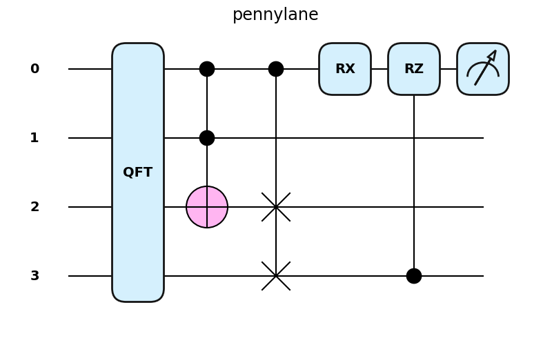
Circuit drawings and plots can now be created following a PennyLane style. (#3950)

The qml.draw_mpl function accepts a style='pennylane' argument to create PennyLane themed circuit diagrams:

def circuit(x, z):
    qml.QFT(wires=(0,1,2,3))
    qml.Toffoli(wires=(0,1,2))
    qml.CSWAP(wires=(0,2,3))
    qml.RX(x, wires=0)
    qml.CRZ(z, wires=(3,0))
    return qml.expval(qml.PauliZ(0))

qml.draw_mpl(circuit, style="pennylane")(1, 1)

PennyLane-styled plots can also be drawn by passing "pennylane.drawer.plot" to Matplotlib's plt.style.use function:

import matplotlib.pyplot as plt

plt.style.use("pennylane.drawer.plot")
for i in range(3):
    plt.plot(np.random.rand(10))

If the font Quicksand Bold isn't available, an available default font is used instead.

Making operators immutable and PyTrees

Any class inheriting from Operator is now automatically registered as a pytree with JAX. This unlocks the ability to jit functions of Operator. (#4458)

>>> op = qml.adjoint(qml.RX(1.0, wires=0))
>>> jax.jit(qml.matrix)(op)
Array([[0.87758255-0.j        , 0.        +0.47942555j],
       [0.        +0.47942555j, 0.87758255-0.j        ]],      dtype=complex64, weak_type=True)
>>> jax.tree_util.tree_map(lambd...

Assets 2

02 Aug 15:36

eddddddy

v0.31.1

0905217

Release 0.31.1

Improvements 🛠

data.Dataset now uses HDF5 instead of dill for serialization. (#4097)
The qchem functions primitive_norm and contracted_norm are modified to be compatible with higher versions of scipy. (#4321)

Bug Fixes 🐛

Dataset URLs are now properly escaped when fetching from S3. (#4412)

Contributors ✍️

This release contains contributions from (in alphabetical order):

Utkarsh Azad, Jack Brown, Diego Guala, Soran Jahangiri, Matthew Silverman

Assets 2

Releases: PennyLaneAI/pennylane

Release 0.36.0

Release 0.36.0

New features since last release

Estimate errors in a quantum circuit 🧮

Access an extended arsenal of quantum algorithms 🏹

Make use of more methods to map from molecules 🗺️

Release 0.35.1

Bug fixes 🐛

Contributors ✍️

Release 0.35.0

New features since last release

Qiskit 1.0 integration 🔌

Native mid-circuit measurements on Default Qubit 💡

Work easily and efficiently with operators 🔧

New Clifford device 🦾

Release 0.34.0.post1

Release 0.34.0

New features since last release

Statistics and drawing for mid-circuit measurements 🎨

Catalyst is seamlessly integrated with PennyLane ⚗️

Decompose circuits into the Clifford+T gateset 🧩

Use an iterative approach for quantum phase estimation 🔄

Release 0.33.1

Bug fixes 🐛

Contributors ✍️

Release 0.33.0

New features since last release

Postselection and statistics in mid-circuit measurements 📌

Exponentiate Hamiltonians with flexible Trotter products 🐖

Building blocks for quantum phase estimation 🧱

New device capabilities, integration with Catalyst, and more! ⚗️

Improvements 🛠

More PyTrees!

Improving QChem and existing algorithms

Release 0.32.0-post1

Release 0.32.0

New features since last release

Encode matrices using a linear combination of unitaries ⛓️️

Monitor PennyLane's inner workings with logging 📃

More input states for quantum chemistry calculations ⚛️

Reuse and reset qubits after mid-circuit measurements ♻️

Improvements 🛠

A new PennyLane drawing style

Making operators immutable and PyTrees

Release 0.31.1

Improvements 🛠

Bug Fixes 🐛

Contributors ✍️