DATASET (kaggle): Web page Phishing Detection Dataset
This dataset, as described on the Kaggle website, is formed mostly by data that has been extracted directly from the structure and syntax of different URLs, as well as from content of their corresponding websites and information collected by querying external services.
The dataset consists of 11430 unique samples with 89 attributes:
- 31 represent categorical data. In fact, all of them are binary variables. The objective variable (status) is included here.
- 1 that contains the whole URL.
- 55 are numerical data, most in the form of counts or averages.
The main goal is to find a classification model based on a supervised learning algorithm that can detect if a website is being used for phishing or not. To compare different candidates, the accuracy will be used as the main score. The recall and F1-score scores will serve as a secondary source of confidence in the obtained results.
The required time for training will be also considered if it is exceptionally high compared with the rest of results, but having a really fast model is not a priority for this analysis.
To gain an overview of the dataset and it's features, we can do a correlation analysis. This way, we can find those attributes that describe better how the data behaves. The following image shows the 15 better correlated with the objective variable:

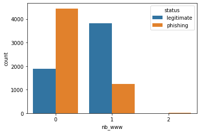
According to the graph, the most correlated features are google_index, page_rank, nb_ww, domain_age and ratio_digits_url. Let's plot them and try to conclude something:

![]()


Just by looking at categorical features like google_index and nb_www it is possible to do a pretty accurate guess about what class a certain sample pertains to. Numerical attributes like page_rank, domain_age or ratio_digits_url, although in the boxplot the two classes overlap, we can see how most of the legitimate samples are closer to their mean than the phishing samples are.
We can also do a PCA (more on that later) and represent the first two principal components. This way we can check if the previous suppositions have any sense when we take into account all the features from the dataset.

As we thought, the legitimate samples tend to be closer (have less variance) than the phishing ones. If we do the same with 3 components, the results are the same.
Two different machine learning algorithms have been used for the analysis:
-
A logistic regression model implemented with PyTorch
-
Different SVM models with all the different predefined kernels, implemented with scikit-learn:
- Linear kernel.
- RBF (Radial Basis Function) kernel.
- Sigmoid kernel.
- Polynomial kernel (up to 4th degree).
The reason for not using more types of algorithms is that I thought that it would be more interesting to focus on how the experiments related to the preprocessing affect the result. With fewer types of models, I was able to spend more time experimenting with different configurations for two algorithms, instead of covering, with less detail, four or five.
The initial dataset didn't required a lot of preprocessingn regarding missing values or useless data. The only feature that had to be removed was the URL since all the information that can be extracted from it is already collected in the rest of columns.
Also, luckily since we want to perform a binary classification, the samples were evenly split between those labeled as phishing and legitimate (5715 of each, exactly 50%), so in that sense there wasn't any problem related to unbalanced data.
Once that was covered, the first consideration was if feature scaling would represent an improvement in the classification task or not (and also I thought that it would be interesting to see the difference). After training some models for both standardized and non-standardized data, the results showed that the non-standardized models not only got a significantly lower accuracy and recall than the standardized ones (at best, the first ones got 64.2% accuracy while the worst standardized got 86.51%), but also the time needed for the training in some cases was so large (it didn't finish after several hours) that I couldn't find a model for the SVM algorithm with linear and polynomial (1st, 2nd and 3rd degree) kernels.
The last experiment regarding preprocessing was seeing if reducing the dimensions of the data would be beneficial in any way. By this I mean that a model, even with a slightly worse accuracy or F1-score, may be still worth it because the training time is more convenient.
For this purpose I have studied two methods for reducing the dimensions: The first one is performing a feature selection of some kind. For this dataset I decided to do selections based on the Mutual Information between each independent variable and the objective variable. This is a great score function for data that mixes categorical and non-categorical variables, as well as being model neutral (can be applied to different types of ML models) and relatively fast.
Two new datasets were created with feature selection, one with 15 attributes and the other with 30. I chose arbitrarily these number because I was interested in studying the effect of a significant reduction of features (Remember that we began with 87 features). After some tests, the results showed that for both cases, the accuracies, as well as the recalls, were pretty close to the model without feature selection (usually a few tenths behind). Overall the F1-score shown a great performance.
If we take a look at the training times, they were much better, especially with the case with 30 features, consistently improving by 40% to 60% the original time.
The other method for reducing the dimensionality of the dataset is by performing a Principal Component Analysis (PCA). By taking into account the variance of each principal component we can find the number of dimensions (components) that we need to keep in order to ensure a certain amount of the original explained variance. I decided to make two experiments keeping 90% and 95% of that variance, and thus I had to work with 50 and 59 components respectively.
The results regarding scores were very close to the standardized dataset for the case with 90% of explained variance, but the training time varies greatly depending on the model, in some cases lasting several minutes, and if we also add the time spent doing the PCA we are left with hardly any room for improvement in any case.
For the case with 95%, althought there are some problems with the training times for some models, others not only are relatively fast, but also have accuracy scores higher than the standardized dataset model.
For all the different models an hyperparameter search has been done, most of them being the result of random searches of 200 iterations each. For the SVM models of 2nd, 3rd and 4th degree, the number of iterations was reduced to 50 because some combinations of hyperparameters caused very long training times.
Also, some cross-validation (K-Fold) was introduced for validating the results. For the logistic regression the number of folds was found as part of the hyperparameter search, while for the SVM models it was set from the beginning: The ones with a polynomial kernel of 2nd, 3rd and 4th degree used 10 folds in order to prevent overfitting the data (The accuracy for the test sets was greater than 99%). The rest used 3 folds.
The following 7 models are a selection of the most relevant models that I have found.
The first three, although with a slightly worse accuracy than the rest, have a very fast training time. The rest are slower (but still fast compared to other models) but have great accuracy scores.
The accuracy scores and training times for all the previous experiments are gathered in the scores.txt file. Also, the same models are saved in the models folder and can be loaded using the functions provided (See Demo).
| Model | Details |
Hyperparameters |
Accuracy | Recall |
F1-score | Time |
|---|---|---|---|---|---|---|
| Logistic Regression | 30 features (FS) |
|
93.43% | 93.1934% | 0.935206 | 2.5324s |
| SVM | Linear kernel |
|
94.716% | 94.8562% | 0.947052 | 4.1421s |
| SVM | RBF kernel, 15 features (FS) |
|
94.436% | 93.9424% | 0.944656 | 3.9144s |
| SVM | Polynomial kernel (2nd deg.) |
|
95.617% | 95.9644% | 0.956012 | 22.2996s |
| SVM | Polynomial kernel (2nd deg.), PCA (95% explained variance) |
|
95.932% | 96.2713% | 0.959198 | 35.3752s |
| SVM | Polynomial kernel (2nd deg.), PCA (90% explained variance) |
|
95.311% | 95.7489% | 0.953695 | 16.2763s |
| SVM | Polynomial kernel (3nd deg.), 30 features (FS) |
|
95.188% | 95.428% | 0.951746 | 14.8542s |
For training and saving new models, follow the example in demo/training.py. By running the next command you can create some Test models:
python demo/train_models.py
There are already trained models saved in this repository. The example provided in demo/scoring.py show how to do this. Use the following command to score the Test models:
python demo/scorin.py
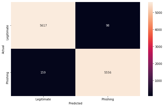
The best model obtained has been the SVM model with a 2nd degree polynomial kernel. This decision comes from it having the best accuracy score (95.932%), which is confirmed to be consistent by the recall (96.2713%) and F1-score (0.959198) scores. The training time (35.3752s) is higher than the rest of the selected models but, since it is still good, and we don't necessarily need a fast model, I have decided to stick to the plain performance regarding the results of the algorithm.
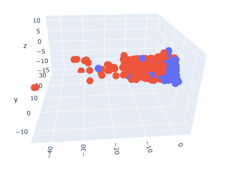
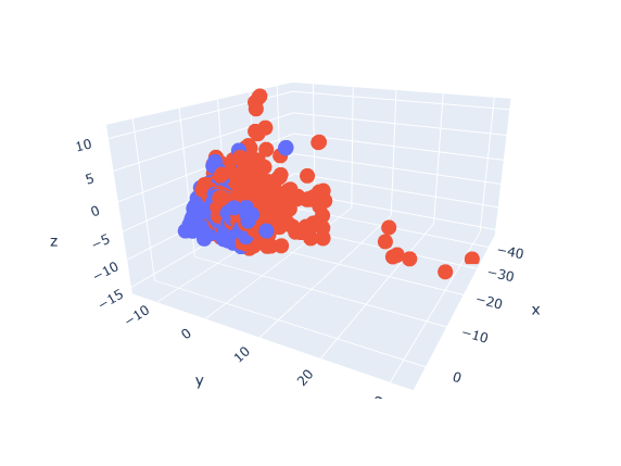
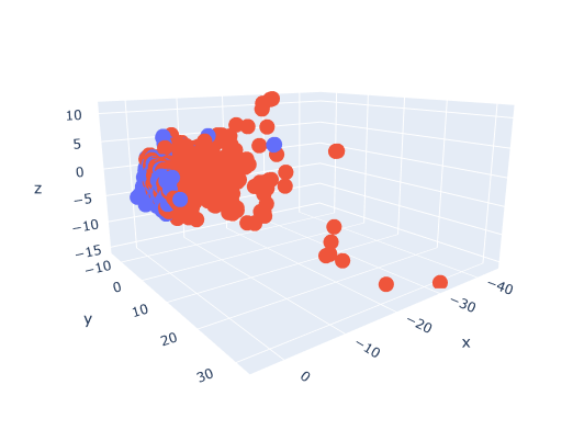
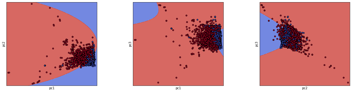
As an example of how the classification with this model works, the following graphics show, firstly, a confusion matrix of the predictions against the real labels of all the samples of the dataset and, below that, three images with the decision boundary that the algorithm builds between the first three principals components along with all the samples ("Phishing" in red, "Legitimate" in blue).
Overall, the results of this analysis are concluding, and I am satisfied with the accuracy obtained. Still, I want to say that the selection of the final model was really hard due to the closeness of the rest of models and, in a different context, maybe some other could have been accepted.
I have found interesting the fact that for almost every experiment regarding preprocessing that I have performed, it was possible to find a correct configuration of hyperparameters that produced an acceptable model.
-
Test the difference between normalizing or standardizing the data.
-
Work with different score functions in the feature selection.
-
Use kernels of my own (Gaussian kernel, Laplace RBF kernel, etc.) in the SVM models.
-
Implement some kind of neural network (and overall use more features from PyTorch)
-
Be able to save actual trained models instead of just configurations of hyperparameters. I was able to do that in the firsts versions of the code, but I got some problems after introducing K-Fold and decided to implement the current solution.
-
Use classes with methods and attributes instead of functions.