54 Fundamental Computer Vision Interview Questions

You can also find all 54 answers here 👉 Devinterview.io - Computer Vision

1. What is computer vision and how does it relate to human vision?

Computer Vision, a branch of Artificial Intelligence, aims to enable computers and machines to interpret and understand visual information such as images and videos. The field draws inspiration from the human visual system to replicate similar functions in machines.

Mimicking Human Vision

By emulating the visual faculties present in humans, Computer Vision tasks can be broken down into several steps, each corresponding to a particular function or mechanism observed in the human visual system.

These steps include:

1. Visual Perception: Taking in visual information from the environment. In the case of machines, data is acquired through devices like cameras.

2. Feature Extraction: Identifying distinctive patterns or characteristics in the visual data. In humans, this involves encoding visual information in the form of object contours, textures, and colors. For machines, this may involve techniques such as edge detection or region segregation.

3. Feature Representation and Recognition: This encompasses grouping relevant features and recognizing objects or scenes based on these features. In the context of artificial systems, this is achieved through sophisticated algorithms such as neural networks and support vector machines.

4. Data Analysis and Interpretation: Understanding objects, actions, and situations in the visual context. This step can involve multiple layers of processing to extract detailed insights from visual data, similar to how the human brain integrates visual input with other sensory information and prior knowledge.

Human and Computer Vision: A Comparison

	Human Vision	Computer Vision
Data Input	Sensed by eyes, then registered and processed by the brain	Captured through cameras and video devices
Hardware	Eyes, optic nerves, and the visual cortex	Cameras, storage devices, and processors (such as CPUs or GPUs)
Perception	Real-time visual comprehension with recognized patterns, depth, and motion	Data-driven analysis to identify objects, classify scenes, and extract features
Object Recognition	Contextual understanding with the ability to recognize familiar or unfamiliar objects based on prior knowledge	Recognition based on statistical models, trained on vast amounts of labeled data
Robustness	Adapts to varying environmental conditions, such as lighting changes and occlusions	Performance affected by factors like lighting, image quality, and occlusions
Educative Process	Gradual learning and refinement of vision-related skills from infancy to adult stages	Continuous learning through exposure to diverse visual datasets and feedback loops

Challenges and Advancements

While modern-day Computer Vision systems have made significant strides in understanding visual information, they still fall short of replicating the speed, flexibility, and generalization observed in human vision.

Researchers in the field continue to work on developing innovative algorithms and improving hardware capabilities to address challenges like visual clutter, three-dimensional scene understanding, and complex context recognition, aiming for systems that are not only efficient but also reliable and adaptable in diverse real-world scenarios.

2. Describe the key components of a computer vision system.

A Computer Vision (CV) system processes and interprets visual data to make decisions or disambiguate tasks. These systems perceive, understand, and act on visual information, much like the human visual system.

The components of a Computer Vision System generally include tasks such as Image Acquisition, Pre-processing, Feature Extraction, Image Segmentation, Object Recognition, and Post-processing.

Key Components

Input Device

The Image Acquisition module typically interfaces with devices such as smartphones, digital cameras, or webcams. In some cases, it may access pre-recorded video or static images.

Data Pre-processing

This stage standardizes the input data for robust processing. Techniques like noise reduction, contrast enhancement, and geometric normalization ensure quality data.

Feature Extraction

The system identifies key visual attributes for analyzing images. Methods can range from basic edge detection and corner detection to more advanced techniques powered by deep neural networks.

Segmentation

This component divides the image into meaningful segments or regions for clearer analysis, doing tasks such as identifying individual objects or distinguishing regions of interest.

• Object Recognition: Utilizes advanced algorithms for detecting and classifying objects within the image. Common methods include template matching, cascade classifiers, or deep learning networks such as R-CNN, YOLO, or SSD.

• 3D Modeling: This optional step constructs a 3D representation of the scene or object.

Decision and Action

Upon analyzing the visual input, the system makes decisions or takes actions based on its interpretation of the data.

Post-processing

The Post-Processing module cleans, clarifies, and enhances the identified information or assessed scene, to improve task performance or user interpretation.

3. Explain the concept of image segmentation in computer vision.

Image Segmentation involves dividing a digital image into multiple segments (sets of pixels) to simplify image analysis.

Techniques

1. Intensity-based Segmentation: Segments based on pixel intensity.
2. Histogram Thresholding: Segments via pixel intensity histograms.
3. Color-based Segmentation: Segments based on color.
4. Edge Detection: Segments by identifying edges.
5. Region Growing: Segments by adjacent pixel similarity.

Challenges

• Over-segmentation: Too many segments making analysis complex.
• Under-segmentation: Loss of detail.
• Noise Sensitivity: Sensitive to image noise.
• Shadow and Highlight Sensitivity: Segments shaded and highlighted areas inconsistently.

Metrics for Evaluation

• Jaccard Index: Measures similarity between sets.
• Dice Coefficient: Measures the spatial overlap between two segments.
• Relative Segmentation Accuracy: Quantifies success based on correctly segmented pixels.
• Probabilistic Rand Index: A statistical measure of the similarity between two data clusters.

Code Example: K-means Segmentation

Here is the Python code:

import numpy as np
import cv2

# Load image
image = cv2.imread('example.png')

# Convert to RGB (if necessary)
image = cv2.cvtColor(image, cv2.COLOR_BGR2RGB)

# Flatten to 2D array
pixels = image.reshape(-1, 3).astype(np.float32)

# Define K-means parameters
criteria = (cv2.TERM_CRITERIA_EPS + cv2.TERM_CRITERIA_MAX_ITER, 100, 0.2)
k = 3

# Apply K-means
_, labels, centers = cv2.kmeans(pixels, k, None, criteria, 10, cv2.KMEANS_RANDOM_CENTERS)

# Reshape labels to the size of the original image
labels = labels.reshape(image.shape[0], image.shape[1])

# Create k segments
segmented_image = np.zeros_like(image)
for i in range(k):
    segmented_image[labels == i] = centers[i]

# Display segments
plt.figure()
plt.imshow(image)
plt.title('Original Image')
plt.show()

plt.figure()
plt.imshow(segmented_image)
plt.title('Segmented Image')
plt.show()

4. What is the difference between image processing and computer vision?

While Image Processing and Computer Vision share some common roots and technologies, they serve distinct purposes.

Image Processing

• Definition: Image processing involves the processing of an image to enhance or extract information.
• Objective: The goal here is to improve image data for human interpretation or storage efficiency.
• Focus: Image processing is typically concerned with pixel-level manipulations.
• Main Tools: Image processing often uses techniques such as filtering, binarization, and noise reduction.
• Applications: Common applications include photo editing, document scanning, and medical imaging.

Computer Vision

• Definition: Computer vision encompasses the automatic extraction, analysis, and understanding of information from images or videos.
• Objective: The aim is to make meaning from visual data, enabling machines to comprehend and act based on what they "see."
• Focus: Computer vision works at a higher level, processing information from an entire image or video frame.
• Main Tools: Computer vision makes use of techniques such as object detection, feature extraction, and deep learning for image classification and segmentation.
• Applications: Its applications are diverse, ranging from self-driving cars and augmented reality to systems for industrial quality control.

5. How does edge detection work in image analysis?

Edge detection methods aim to find the boundaries in images. This step is vital in various computer vision tasks, such as object recognition, where edge pixels help define shape and texture.

Types of Edges in Images

Modern edge detection methods are sensitive to various types of image edges:

• Step Edges: Rapid intensity changes in the image.
• Ramp Edges: Gradual intensity transitions.
• Roof Edges: Unidirectional edges associated with a uniform image region.

Sobel Edge Detection Algorithm

The Sobel operator is one of the most popular edge detection methods. It calculates the gradient of the image intensity by convolving the image with small[ square 3x3 convolution kernels][4]. One for detecting the x-gradient and the other for the y-gradient.

These kernels are:

$G_x$

$$ G_x = \begin{bmatrix} +1 & 0 & -1 \\ +2 & 0 & -2 \\ +1 & 0 & -1 \end{bmatrix} $$

$G_y$

$$ G_y = \begin{bmatrix} +1 & +2 & +1 \\ 0 & 0 & 0 \\ -1 & -2 & -1 \end{bmatrix} $$

The magnitude $G$ and direction $\theta$ of the gradient are then calculated as:

$$ G = \sqrt{G_x^2 + G_y^2} $$

$$ \theta = \arctan\left(\frac{G_y}{G_x}\right) $$

The calculated $G$ and $\theta$ are used to detect edges.

Canny Edge Detection

The Canny edge detector is a multi-step algorithm which can be outlined as follows:

1. Noise Reduction: Apply a Gaussian filter to smooth out the image.
2. Gradient Calculation: Use the Sobel operator to find the intensity gradients.
3. Non-Maximum Suppression: Thins down the edges to one-pixel width to ensure the detection of only the most distinct edges.
4. Double Thresholding: To identify "weak" and "strong" edges, pixels are categorized based on their gradient values.
5. Edge Tracking by Hysteresis: This step defines the final set of edges by analyzing pixel gradient strengths and connectivity.

Implementations in Python

Here is the Python code:

Using Canny Edge Detection from OpenCV

import cv2

# Load the image in grayscale
img = cv2.imread('image.jpg', 0)

# Apply Canny edge detector
edges = cv2.Canny(img, 100, 200)

# Display the original and edge-detected images
cv2.imshow('Original Image', img)
cv2.imshow('Edges', edges)
cv2.waitKey(0)
cv2.destroyAllWindows()

Using Sobel Operator from OpenCV

import cv2
import numpy as np
from matplotlib import pyplot as plt

# Load the image in grayscale
img = cv2.imread('image.jpg', 0)

# Compute both G_x and G_y using the Sobel operator
G_x = cv2.Sobel(img, cv2.CV_64F, 1, 0, ksize=3)
G_y = cv2.Sobel(img, cv2.CV_64F, 0, 1, ksize=3)

# Compute the gradient magnitude and direction
magnitude, direction = cv2.cartToPolar(G_x, G_y)

# Display the results
plt.subplot(121), plt.imshow(magnitude, cmap='gray')
plt.title('Gradient Magnitude'), plt.xticks([]), plt.yticks([])
plt.subplot(122), plt.imshow(direction, cmap='gray')
plt.title('Gradient Direction'), plt.xticks([]), plt.yticks([])
plt.show()

6. Discuss the role of convolutional neural networks (CNNs) in computer vision.

Convolutional Neural Networks (CNNs) have revolutionized the field of computer vision with their ability to automatically and adaptively learn spatial hierarchies of features. They are at the core of many modern computer vision applications, from image recognition to object detection and semantic segmentation.

CNNs Hierarchy of Layers

• Input Layer: Often a matrix representation of pixel values.
• Convolutional Layer: Utilizes a series of learnable filters for feature extraction.
• Activation Layer: Typically employs ReLU, introducing non-linearity.
• Pooling Layer: Subsambles spatial data, reducing dimensionality.
• Fully Connected Layers: Classic neural network architecture for high-level reasoning.

Key Operations

Convolution

1. Local Receptive Field: Small portions of the image are convolved with the filter, which is advantageous for capturing local features.
2. Parameter Sharing: A single set of weights is employed across the entire image, reducing the model's training parameters significantly.

Pooling

1. Downsampling: This process compresses the spatial data, making the model robust to variations in scale and orientation.
2. Invariance: By taking, for instance, the average or maximum pixel intensity in a pooling region, pooling layers display invariance toward small translations.

Feature Hierarchy

Each convolutional layer, in essence, stacks its learned features from preceding layers. Early layers are adept at edge detection, while deeper layers can interpret these edges as shapes or even complex objects.

Global Receptive Field

With every subsequent convolutional layer, the receptive field—the portion of the input image influencing a neuron's output—expands. This expansion enables the network to discern global relationships from intricate local features.

Regularization & Overfitting

CNNs inherently offer overfitting avoidance through techniques like pooling and, more importantly, data augmentation, thereby enhancing their real-world adaptability. Moreover, dropout and weight decay are deployable regularizers to curb overfitting, particularly in tasks with limited datasets.

Automated Feature Hierarchy Construction

CNNs distinctly differ from traditional computer vision methods that require manual feature engineering. CNNs automate this process, a characteristic vital for intricate visual tasks like object recognition.

Real-Time Applications

CNNs undergird a profusion of practical implementations ranging from predictive policing with video data to hazard detection in autonomous vehicles. Their efficacy in these real-time scenarios is primarily due to their architecture's efficiency at processing visual information.

7. What's the significance of depth perception in computer vision applications?

Depth perception is crucial in various computer vision tasks, improving localization precision, object recognition, and 3D reconstruction.

Core Functions Enabled by Depth Perception

Segmentation

Depth assists in separating foreground objects from the background, crucial in immersive multimedia, robotics, and precision motion detection.

Object Recognition

Incorporating depth enhances the precision of object recognition, especially in cluttered scenes, by offering valuable spatial context.

3D Scene Understanding

Depth data enables the accurate arrangement and orientation of objects within a scene.

Image Enhancement

Computing depth can lead to image enhancements such as depth-based filtering, super-resolution, and scene orientation corrections.

Human-Machine Interaction

Understanding depth leads to more user-friendly interfaces, especially in augmented reality and human-computer interaction applications.

Visual Effects

Depth contributes to realistic rendering of virtual objects in live-action scenes. Its role in producing immersive 3D experiences in movies, games, and virtual reality is undeniable.

Techniques for Depth Estimation

Monocular Depth Estimation

Monocular depth is classified into five categories:

• From cues: Depth is inferred from indications like occlusions and textures.
• From defocus: Depth is assessed from changes in focus, observed in systems like light field cameras.
• From focus: Depth is deduced based on varying sharpness.
• From behavioral cues: Depth is gauged using prior knowledge about object attributes like size or motion.
• Features: Modern methods often leverage CNN-based estimators.

Binocular Depth Estimation

Binocular vision includes:

• Disparity: Depth is inferred from discrepancies in object position between the left and right camera perspectives.
• Shape from shading: Depth is extracted by assessing object surface topography from differing lighting angles.

Multiview Depth Estimation

By fusing depth observations from various viewpoints, multiview methods offer improved depth precision and can often address occlusion challenges.

RGBD

The combination of depth data from sensors like the Kinect with traditional RGB images.

Time-of-Flight and Structured Light

These approaches include sensors that estimate depth based on the time light takes to travel to an object and back, or the deformation of projected light patterns.

LiDAR and Stereo Camera Systems

LiDAR scans scenes with laser light, while stereo vision systems ascertain depth from the discrepancy between paired camera views.

8. Explain the challenges of object recognition in varied lighting and orientations.

Object recognition, which involves identifying and categorizing objects in images or videos, can be challenging in several ways, especially with variations in lighting and object orientation.

Key Challenges

1. Occlusion: Objects might be partially or completely hidden, making accurate identification difficult.

2. Varying Object Poses: Different orientations, such as tilting, rotating, or turning, can make it challenging to recognize objects.

3. Background Clutter: Contextual noise or cluttered backgrounds can interfere with identifying objects of interest.

4. Intra-Class Variability: Objects belonging to the same class can have significant variations, making it hard for the model to discern common characteristics.

5. Inter-Class Similarities: Objects from different classes can share certain visual features, leading to potential misclassifications.

6. Lighting Variations: Fluctuations in ambient light, such as shadows or overexposure, can distort object appearances, affecting their recognition.

7. Perspective Distortions: When objects are captured from different viewpoints, their 2D representations can deviate from their 3D forms, challenging recognition.

8. Visual Obstructions: Elements like fog, rain, or steam can obscure objects in the visual field, hindering their identification.

9. Resolution and Blurring: Images with low resolution or those that are blurry might not provide clear object details, impacting recognition accuracy.

10. Semantic Ambiguity: Subtle visual cues, or semantic ambiguities, can make it challenging to differentiate and assign the correct label among visually similar objects.

11. Mirror Images: Object recognition systems should ideally be able to distinguish between an object and its mirror image.

12. Textured Surfaces: The presence of intricate textures can sometimes confuse recognition algorithms, especially when shapes are:

    • 3D
    • Convex
    • Large in size

13. Speed and Real-Time Constraints: The requirement for rapid object recognition, such as in automated manufacturing or self-driving cars, poses a challenge in ensuring quick and accurate categorization.

Techniques to Address Challenges

• Data Augmentation: Generating additional training data by applying transformations like rotations, flips, and slight brightness or contrast adjustments.

• Feature Detectors and Descriptors: Utilizing algorithms like SIFT, SURF, or ORB for reliable feature extraction and matching, enabling robustness against object orientation and background clutter.

• Pose Estimation: Using methods like the Perspective-n-Point (PnP) algorithm, which takes 2D-3D correspondences to estimate the pose (position and orientation) of an object.

• Advanced Learning Architectures: Employing state-of-the-art convolutional neural networks (CNNs), such as ResNets and Inception Net, that are adept at learning hierarchical features, leading to better recognition in complex scenarios.

• Ensemble Methods: Harnessing the collective wisdom of multiple models, which can be beneficial in addressing challenges such as lighting variations and partial occlusions.

• Transfer Learning: Leveraging the knowledge acquired from pre-trained models on vast datasets to kick-start object recognition tasks. This can be instrumental in reducing the need for prohibitively large datasets for training.

9. What are the common image preprocessing steps in a computer vision pipeline?

Image pre-processing involves a series of techniques tailored to optimize images for computer vision tasks such as classification, object detection, and more.

Steps in Pre-processing

1. Image Acquisition: Retrieving high-quality images from various sources, including cameras and databases.

2. Image Normalization: Standardizing image characteristics like scale, orientation, and color.

3. Noise Reduction: Strategies for minimizing noise or distorted information that affects image interpretation.

4. Image Enhancement: Techniques to improve visual quality and aid in feature extraction.

5. Image Segmentation: Dividing images into meaningful segments, simplifying their understanding.

6. Feature Extraction: Identifying and isolating critical features within an image.

7. Feature Selection: Streamlining models by pinpointing the most relevant features.

8. Data Splitting: Partitioning data into training, validation, and test sets.

9. Dimensionality Reduction: Techniques for lowering feature space dimensions, particularly valuable for computationally intensive models.

10. Image Compression: Strategies to reduce image storage and processing overheads.

Code Example: Data Splitting

Here is the Python code:

from sklearn.model_selection import train_test_split

# Split data into training and testing sets
X_train, X_test, y_train, y_test = train_test_split(images, labels, test_size=0.2, random_state=42)

Key Image Pre-processing Techniques

• Resizing: Compressing images to uniform dimensions.
• Filtering: Using various filters to highlight specific characteristics, such as edges.
• Binarization: Converting images to binary format based on pixel intensity, simplifying analysis.
• Thresholding: Dividing images into clear segments, often useful in object detection.
• Image Moments: Abstract data to describe various properties of image data, such as the center or orientation.
• Feature Detection: Automatically identifying and marking key points or structures, like corners or lines.
• Histogram Equalization: Improving image contrast by altering intensity distributions.
• ROI Identification: Locating regions of interest within images, helping focus computational resources where they're most needed.

Image Pre-Processing for Specific Tasks

1. Classification: Tasks images into predefined classes.

   • Techniques: Center-cropping, mean subtraction, PCA color augmentation.

2. Object Detection: Identifies and locates objects within an image.

   • Techniques: Resizing to anchor boxes, data augmentation.

3. Semantic Segmentation: Assigns segments of an image to categories.

   • Techniques: Image resizing to match the model's input size, reprojection of results.

4. Instance Segmentation: Identifies object instances in an image while categorizing and locating pixels related to each individual object.

   • Techniques: Scaling the image, padding to match network input size.

10. How does image resizing affect model performance?

Image resizing has substantial implications for both computational efficiency and model performance in computer vision applications. Let's delve into the details.

Impact on Convolutional Neural Networks

Convolutional Neural Networks (CNNs) are the cornerstone of many computer vision models due to their ability to learn and detect features hierarchically.

Benefit of Image Resizing for Efficiency

1. Computational Efficiency: Resizing reduces the number of operations. Fewer pixels mean a shallower network may suffice without losing visual context.
2. Memory Management: Smaller images require less memory, often fitting within device constraints.

Drawbacks of Resizing

1. Information Loss: Shrinking images discards fine-grained details crucial in image understanding.
2. Sparse Receptive Field Coverage: Small input sizes can limit receptive fields, compromising global context understanding.
3. Overfitting Risk: Extreme reductions can cause overfitting, especially with simpler models and limited data.

Tackling the Information Loss

• Data Augmentation: Introduce image variations during training.
• Progressive Resizing: Start with smaller images, progressing to larger ones.
• Mixed Scaled Batches: Train using a mix of image scales in each batch.

Optimal Input Sizes

Establishing an optimal input size involves considering computational constraints and the need for high-resolution feature learning.

For real-time applications, such as self-driving cars, quick diagnostic systems, or embedded devices, practicality often demands smaller image sizes. Conversely, for image-specific tasks where detailed information is crucial, such as in pathology or astronomical image analysis, larger sizes are essential.

Code Example: Image Resizing

Here is the Python code:

import cv2

# Load an image
image = cv2.imread('path_to_image.jpg')

# Resize to specific dimensions
resized_image = cv2.resize(image, (new_width, new_height))

# Display
cv2.imshow("Original Image", image)
cv2.imshow("Resized Image", resized_image)
cv2.waitKey(0)
cv2.destroyAllWindows()

11. What are some techniques to reduce noise in an image?

Image noise can disrupt visual information and hinder both human and machine perception. Employing effective noise reduction techniques can significantly improve the quality of images.

Common Image Noise Types

• Gaussian Noise: Results from the sum of many independent, tiny noise sources. Noise values follow a Gaussian distribution.
• Salt-and-Pepper Noise: Manifests as random white and black pixels in an image.

Techniques for Noise Reduction

Median Filter

The median filter replaces the pixel value with the median of the adjacent pixels. This method is especially effective for salt-and-pepper noise.

Gaussian Filter

The Gaussian filter uses a weighted averaging mechanism, giving more weight to pixels closer to the center.

Bilateral Filter

The bilateral filter also uses a weighted averaging technique, with two key distinctions: it considers spatial closeness and relative intensities.

Non-local Means Filter (NLM)

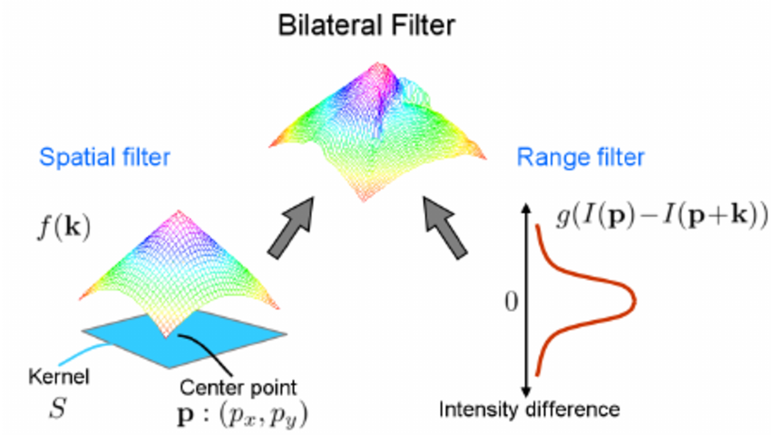
The NLM filter compares similarity between patches in an image to attenuate noise.

Code Example: Common Noise Reduction Filters

Here is the Python code:

import cv2
import matplotlib.pyplot as plt

# Read image and convert to grayscale
image = cv2.imread('noisy_image.png')
gray = cv2.cvtColor(image, cv2.COLOR_BGR2GRAY)

# Apply different noise reduction filters
median_filtered = cv2.medianBlur(gray, 5)
gaussian_filtered = cv2.GaussianBlur(gray, (5, 5), 0)
bilateral_filtered = cv2.bilateralFilter(gray, 9, 75, 75)

# Display all images
plt.figure(figsize=(10, 5))
plt.subplot(2, 2, 1), plt.imshow(gray, cmap='gray')
plt.title('Original'), plt.xticks([]), plt.yticks([])
plt.subplot(2, 2, 2), plt.imshow(median_filtered, cmap='gray')
plt.title('Median Filter'), plt.xticks([]), plt.yticks([])
plt.subplot(2, 2, 3), plt.imshow(gaussian_filtered, cmap='gray')
plt.title('Gaussian Filter'), plt.xticks([]), plt.yticks([])
plt.subplot(2, 2, 4), plt.imshow(bilateral_filtered, cmap='gray')
plt.title('Bilateral Filter'), plt.xticks([]), plt.yticks([])

plt.show()

12. Explain how image augmentation can improve the performance of a vision model.

Image augmentation is a technique used to artificially enlarge a dataset by creating modified versions of the original images. It helps in improving the accuracy of computer vision models, especially in scenarios with limited or unbalanced data.

Benefits of Image Augmentation

• Improved Generalization: By exposing the model to a range of transformed images, it becomes better at recognizing and extracting features from the input data, making it more robust against variations.

• Data Balancing: Augmentation techniques can be tailored to mitigate class imbalances, ensuring more fair and accurate predictions across different categories.

• Reduced Overfitting: Diverse augmented data presents a variety of input patterns to the model, which can help in preventing the model from becoming overly specific to the training set, thereby reducing overfitting.

Common Augmentation Techniques

1. Geometric transformations: These include rotations, translations, flips, and scaling. For example, a slightly rotated or flipped image can still represent the same object.

2. Color and contrast variations: Introducing color variations, changes in brightness, and contrast simulates different lighting conditions, making the model more robust.

3. Noise addition: Adding random noise can help the model in handling noise present in real-world images.

4. Cutout and occlusions: Randomly removing patches of images or adding occlusions (e.g., a random black patch) can help in making the model more robust to occlusions.

5. Mixup and CutMix: Techniques like mixup and CutMix involve blending images from different classes to create more diverse training instances.

6. Grid Distortion: This advanced technique involves splitting the image into a grid and then perturbing the grid points to create the distorted image.

Code Example: Augmentation with Keras

Here is the Python code:

from keras.preprocessing.image import ImageDataGenerator

# Initialize the generator with specific augmentation parameters
datagen = ImageDataGenerator(
    rotation_range=20,
    width_shift_range=0.2,
    height_shift_range=0.2,
    horizontal_flip=True,
    vertical_flip=True,
    brightness_range=[0.8, 1.2],
    shear_range=0.2,
    zoom_range=0.2,
    fill_mode='nearest')

# Apply the augmentation to an image
import numpy as np
from keras.preprocessing.image import load_img, img_to_array
import matplotlib.pyplot as plt

# Load an example image
img = load_img('path_to_image.jpg')

# Transform the image to a numpy array
data = img_to_array(img)
samples = np.expand_dims(data, 0)

# Create a grid of 10x10 augmented images
plt.figure(figsize=(10, 10))
for i in range(10):
	for j in range(10):
		# Generate batch of images
		batch = datagen.flow(samples, batch_size=1)
		# Convert to unsigned integers for viewing
		image = batch[0].astype('uint8')
		# Define subplot
		plt.subplot(10, 10, i*10+j+1)
		# Plot raw pixel data
		plt.imshow(image[0])
	# Show the plot
plt.show()

13. Discuss the concept of color spaces and their importance in image processing.

Color spaces are mathematical representations designed for capturing and reproducing colors in digital media, such as images or video. They can have different characteristics, making them better suited for specific computational tasks.

Importance of Color Spaces in Image Processing

• Computational Efficiency: Certain color spaces expedite image analysis and algorithms like edge detection.

• Human Perceptual Faithfulness: Some color spaces mimic the way human vision perceives color more accurately than others.

• Device Independence: Color spaces assist in maintaining consistency when images are viewed on various devices like monitors and printers.

• Channel Separation: Storing color information distinct from luminance can be beneficial. For example, in low-light photography, one may prioritize the brightness channel, avoiding the graininess inherent in the color channels.

• Specialized Uses: Unique color representations are crafted explicitly for niche tasks such as skin tone detection in image processing.

By navigating between color spaces, tailored methods for each step of image processing can be implemented, leading to optimized visual results.

Common Color Spaces

RGB (Red, Green, Blue)

This is the basic color space for images on electronic displays. It defines colors in terms of how much red, green, and blue light they contain.

RGB is device-dependent and not human-intuitive.

HSV (Hue, Saturation, Value)

• Hue: The dominant wavelength in the color (e.g., red, green, blue).
• Saturation: The "purity" of the color or its freedom from white.
• Value: The brightness of the color.

This color space is often used for segmenting object colors. For example, for extracting a specific colored object from an image.

CMYK (Cyan, Magenta, Yellow, Black)

This color system is specifically designed for use with printers. Colors are defined in terms of the amounts of cyan, magenta, yellow and black inks needed to reproduce them.

• C is for cyan
• M is for magenta
• Y is for yellow
• K is for black

YCbCr

This color space represents colors as a combination of a luminance (Y) channel and chrominance (Cb, Cr, or U, V in some variations) channels.

It's commonly used in image and video compression, as it separates the brightness information from the color information, allowing more efficient compression.

Conversion Between Color Spaces

Several libraries and image processing tools offer mechanisms to convert between color spaces. For instance, OpenCV in Python provides the cvtColor() function for this purpose.

Here is the Python code:

import cv2

# Load the image
image = cv2.imread('path_to_image.jpg')

# Convert from BGR to RGB
image_rgb = cv2.cvtColor(image, cv2.COLOR_BGR2RGB)

# Convert from RGB to Grayscale
image_gray = cv2.cvtColor(image_rgb, cv2.COLOR_RGB2GRAY)

# Display the images
cv2.imshow('RGB Image', image_rgb)
cv2.imshow('Grayscale Image', image_gray)

# Close with key press
cv2.waitKey(0)
cv2.destroyAllWindows()

14. What are feature descriptors, and why are they important in computer vision?

In Computer Vision, Feature Descriptors provide a compact representation of the information within an image or an object. They are an essential element in many tasks, such as object recognition, image matching, and 3D reconstruction.

The Role of Feature Descriptors

1. Identification: These descriptors help differentiate features (keypoints or interest points) from the background or other irrelevant points.

2. Invariance: They provide robustness against variations like rotation, scale, and illumination changes.

3. Localization: They offer spatial information that pinpoints the exact location of the feature within the image.

4. Matching: They enable efficient matching between features from different images.

Common Feature Detection Algorithms

1. Harris Corner Detector: Identifies key locations based on variations in intensity.

2. Shi-Tomasi Corner Detector: A refined version of the Harris Corner Detector.

3. SIFT (Scale-Invariant Feature Transform): Detects keypoints that are invariant to translation, rotation, and scale. SIFT is also a descriptor itself.

4. SURF (Speeded-Up Robust Features): A faster alternative to SIFT, also capable of detecting keypoints and describing them.

5. FAST (Features from Accelerated Segment Test): Used to detect keypoints, particularly helpful for real-time applications.

6. ORB (Oriented FAST and Rotated BRIEF): Combines the capabilities of FAST keypoint detection and optimized descriptor computation of BRIEF. It is also an open-source alternative to SIFT and SURF.

7. AKAZE (Accelerated-KAZE): Known for being faster than SIFT and able to operate under various conditions, such as viewpoint changes, significant background clutter, or occlusions.

8. BRISK (Binary Robust and Invariant Scalable Keypoints): Focuses on operating efficiently and providing robustness.

9. MSER (Maximally Stable Extremal Regions): Used for detecting regions that stand out in terms of stability across different views or scales. Stood out for its adaptability to various settings.

10. HOG (Histogram of Oriented Gradients): Brings in information from local intensity gradients, often used in conjunction with Machine Learning algorithms.

11. LBP (Local Binary Pattern): Another method for incorporating texture-related details into feature representation.

Key Descriptors and Their Characteristics

• SIFT: Combines orientation and magnitude histograms.
• SURF: Deploys a grid-based approach and features a speed boost by using Integral Images.
• BRIEF (Binary Robust Independent Elementary Features): Produces binary strings.
• ORB: Uses FAST for keypoint detection and deploys a modified version of BRIEF for descriptor generation.

Code Example: Harris Corner Detection

Here is the Python code:

import cv2
import numpy as np

# Load the image in grayscale
image = cv2.imread('house.jpg', 0)

# Set minimum threshold for Harris corner detector
thresh = 10000

# Detect corners using Harris Corner Detector
corner_map = cv2.cornerHarris(image, 2, 3, 0.04)

# Mark the corners on the original image
image[corner_map > 0.01 * corner_map.max()] = [0, 0, 255]

# Display the image with corners
cv2.imshow('Harris Corner Detection', image)
cv2.waitKey(0)
cv2.destroyAllWindows()

15. Explain the Scale-Invariant Feature Transform (SIFT) algorithm.

Scale-Invariant Feature Transform (SIFT) is a widely-used method for keypoint detection and local feature extraction. It's robust to changes like scale, rotation, and illumination, making it effective for tasks such as object recognition, image stitching, and 3D reconstruction.

Core Steps

1. Scale-space Extrema Detection: Identify potential keypoints across multi-scale image pyramids to be robust to scale changes. The algorithm detects extrema in the DoG function.

2. Keypoint Localization: Refine the locations of keypoints using a Taylor series expansion, allowing for sub-pixel accuracy. This step also filters out low-contrast keypoints and poorly-localized ones.

3. Orientation Assignment: Assigns an orientation to each keypoint. This makes the keypoints invariant to image rotation.

4. Keypoint Descriptor: Compute a feature vector, referred to as the SIFT descriptor, which encodes the local image gradient information in keypoint neighborhoods. This step enables matching despite changes in viewpoint, lighting, or occlusion.

5. Descriptor Matching: Compares feature vectors among different images to establish correspondences.

SIFT vs. Modern Techniques

While SIFT has long been a staple in the computer vision community, recent years have introduced alternative methods. For instance, convolutional neural networks (CNNs) are increasingly being used to learn discriminative image features, especially due to their effectiveness in large-scale, real-world applications.

Deep learning-based methods have shown superior performance in various tasks, challenging SIFT's historical dominance. The effectiveness of SIFT, however, endures in many scenarios, particularly in instances with smaller datasets or specific requirements for computational efficiency.

Code Example: SIFT Using OpenCV

Here is the Python code:

# Import the required libraries
import cv2

# Load the image in grayscale
image = cv2.imread('image.jpg', 0)

# Create an SIFT object
sift = cv2.SIFT_create()

# Detect keypoints and descriptors
keypoints, descriptors = sift.detectAndCompute(image, None)

# Visualize the keypoints
image_with_keypoints = cv2.drawKeypoints(image, keypoints, None)
cv2.imshow('Image with Keypoints', image_with_keypoints)
cv2.waitKey(0)
cv2.destroyAllWindows()

Explore all 54 answers here 👉 Devinterview.io - Computer Vision