Ch8-Optimization.md

Ch8: Optimization for Deep Learning

Introduction

• Overall goal: find parameters $\theta$ of a neural network that optimize a defined cost function $J(\theta)$
  • $J$ is generally some quantification of our "performance" over the training data as well as additional regularization terms
• In actuality, we'd like to minimize $$J(\theta) = \mathbb{E}{(x,y) \tilde{} p{data}} L(f(x;\theta), y) = \int_{(x, y) \in{D}}{L(f(x;\theta), y)p(x,y)}$$
  • This is the loss across the entire data generating distrbution, and is intractable, since we don't have access to the data generating distribution
  • This quantity is also known as the "risk"

Empirical Risk Minimization

• We approximate the above quantity by minimizing across the training data: $$\frac{1}{m}\sum_{i=1}^{m} L(f(x_i;\theta), y_i)$$
  • This is known as the empirical risk, since it is computed across the data we have observed, which is a subset of the actual data
    • We can show that the expectation of the empirical risk across the data generating distribution is an unbiased estimate of the true risk: $$\mathbb{E}D[\frac{1}{m}\sum{i=1}^{m} L(f(x_i;\theta), y_i)] = \frac{1}{m}\mathbb{E_D}\sum_{i=1}^{m} L(f(x_i;\theta), y_i)$$
    • By linearity of expectation, we have $$\frac{1}{m}\sum_{i=1}^{m}\mathbb{E_D}[ L(f(x_i;\theta), y_i)]$$
    • Since we use IID assumptions, this is the same as calculating the expectation for any sample from the data generating distribution: $$\frac{1}{m}\sum_{i=1}^{m}\mathbb{E_D}[ L(f(x;\theta), y)]$$, making the sum term the same as the true risk.
    • This result provides us some assurance that empirical risk minimization is a good strategy to also approximate minimizing the true risk, though we can also show that there exist learners for which the true risk is $1$ and the empirical risk is $0$.
      • This is because the result states nothing about the variance of the empirical risk.
• If $$L$$ is the 0-1 loss, then we generally cannot use this function directly, since optimizing on it is intractable.s
• To work around this, a surrogate loss function is often used, such as the negative log-likelihood, as an approximation for the 0/1 loss.
• We can also compute the 0/1 loss across validation data during training, and when it stops decreasing it may be an indication for early stopping.

Batch/minibatch learning

• If we formulate our loss and gradient as the expectation across the # of training examples, this will be expensive, due to large training set sizes
• Using batches of smaller size is faster, and provides many advantages:
  • Accuracy of the gradient is not too much worse- the standard error of the mean is $\frac{\sigma}{\sqrt(n)}$ , meaning that there is less than a linear improvement in the gradient accuracy with more samples.
  • Minibatch learning accounts for redundancy and introduces more stochasticity into the model, has a regularizing effect
  • If examples are not repeated, then it can be shown that minibatch SGD provides an unbiased estimate of the gradient of the generalization error - see pg. 278 of the DLB for a derivation of this.
• If you have smaller batches, you may want to use a smaller learning rate, since the gradient has more variability, and you are "less confident" about taking a larger step in that direction.

Issue w/Optimization: Ill-Conditioning

• Said to happen when the Hessain $H$ is large compared to the gradient norm, and even a very small step in the direction of the gradient would actually increase the cost function rather than decreasing it as desired
• How to find ill conditioning: the Taylor series expansion. Recall that we can have a 2nd order approximation of $f$ at $x_0$: $f(x) \approx f(x_0) + f'(x_0)(x - x_0) + \frac{1}{2}f''(x_0)(x-x_0)^2$. If we let $\textbf{g}$ denote the first derivative and $\textbf{H}$ denote the 2nd derivative, then we have $f(x)\approx f(x_0) + (x-x_0)\textbf{g} + \frac{1}{2}(x-x_0)^T\textbf{H}(x-x_0)$. where $x$ and $x_0$ are now vector-valued.
• The normal gradient descent update would give us $$f(x_0-\epsilon g) \approx f(x_0) + (x_0 - \epsilon g - x_0)g + \frac{1}{2}(x_0 - \epsilon g - x_0)^T\textbf{H}(x_0 - \epsilon g - x_0) $$ $$ = f(x_0) -\epsilon g^Tg+\frac{1}{2}\epsilon^2g^T\textbf{H}g $$
• For gradient descent to give us a smaller value for $f$, we require $$-\epsilon g^Tg+\frac{1}{2}\epsilon^2g^T\textbf{H}g < 0$$ or $$\epsilon g^Tg > \frac{1}{2}\epsilon^2g^T\textbf{H}g$$. This tells us that if the Hessian gets too large, then the right hand term may be greater than the left hand term, and thus gradient descent won't actually reduce our cost function.
  • If we note that during training the $$g^T\textbf{H}g$$ term is getting much larger than the $$g^Tg$$ term, we could further scale the learning rate to keep the right hand term smaller.
    • Again, as with most methods using the Hessian, this is not very practical since computing the Hessian is usually prohibitively expensive.

Issue w/Optimization: Saddle Points/Local Minima

• Since neural networks lead to the optimization of highly nonconvex loss functions, optimization algorithms could potentially converge to a local minima with a significantly higher cost than the global minima
• Can test if local minima is a problem in model training by plotting the norm of the gradient —> it was shown that local minima is usually not the problem, since the norm of the gradient is still quite large when convergence occurs, whereas if it was local minima then the gradient would be about 0.
• Saddle points are points with $0$ gradient, but these points are neither a local min or local max
• We can use a generalization of the 2nd derivative test through examining the eigenvalues of the Hessian
• When $\nabla_xf(x) = 0$ and the Hessian is positive definite (all eigenvalues > 0 at that point), then we're at a local min, since the 2nd directional derivative is everywhere positive, and the grad is 0
• Similarly, when the Hessian is negative definite (all eigenvalues < 0) then we're at a local max
• If it's neither, then we're at a saddle point
• Notion of convexity - central to traditional machine learning loss functions - the Hessian needs to be everywhere positive semidefinite, meaning that we should be able to show for a Hessian $H$ and any real vector $z$, $z^T H z &gt; 0$.
• Saddle points are generally problematic for 2nd order optimization algorithms - such as Newton's method, which is only designed to jump to a point with 0 gradient, so it may jump to a saddle point
  • Modifications such as "Saddle-free Newton's method" exists to accomodate for this
• Aside: main idea for "escaping" saddle points:
  • If you have a saddle point that is "well-behaved", then you can possibly use 2nd order methods to escape the saddle points. For example, if you are at or near a point where $\nabla_{x} f(x) = 0$, but the Hessian is not positive definite or negative definite, then you may be at a saddle point. If you can find a direction $u$ (a directional vector) such that $u^THu &lt; 0$, then this indicates that the update $x = x - \epsilon u$ would decrease the value of the objective, and push you out of the saddle point. We can see this with the Taylor series expansion:
    • $$f(x-\epsilon u) \approx f(x) + \nabla_xf(x)(x - \epsilon u - x) + \frac{1}{2}(x - \epsilon u - x)^T\nabla^2f(x)(x - \epsilon u - x)$$
    • Which becomes, since we are assuming $\nabla_x f(x)= 0$, $$f(x) - \frac{1}{2}\epsilon u^T\nabla^2f(x)(-\epsilon)u = f(x) + \frac{1}{2}\epsilon^2u^T\nabla^2f(x)u$$ which is less than $$f(x)$$.
  • This is harder if we don't have access to 2nd order information - which is usually the case since the 2nd order derivative is expensive to compute and is of quadratic size in the dimension of the optimizaiton problem. In these cases, we normally rely on stochastic/perturbed gradient descent which produces a noisy estimate of the gradient, which has been shown to help escape saddle points.

Issue w/Optimization: Cliffs/Exploding Gradients

• The loss function surface may have large step-function like increases, leading to large gradients. But since the gradient is generally used for the direction of steepest descent and not necessarily the amount to step, we can accomodate for large gradients by imposing a gradient clipping rule. This preserves direction but decreases magnitude.

Issue w/Optimization: Long-term dependencies

• The vanishing/exploding activations/gradient problem:
  • Consider a deep feedforward network that just successively multiplies its input by a matrix $W$ $t$ times. If $W$ has an eigendecomposition $W = V\mathbb{diag}(\lambda)V^{-1}$ then $W^t = V\mathbb{diag}(\lambda)^tV^{-1}$, so unless the eigenvalues are all around an absolute value of $1$, we will have the vanishing/exploding activation problem, and the gradient propagating backwards scales similarly.
  • Research into this problem has yielded several techniques, most notably Batch Normalization and weight initialization schemes such as He & Xavier initialization to ensure that activation and gradients have healthy norms throughout the training process. The central idea revolves around ensuring that the variances between successive layers stays at $1$ instead of converging to $0$.
  • Gradient clipping, especially in RNNs, has been shown to alleviate the exploding gradient problem - the gradient is thought of more as a direction to travel in in the optimization landspace, and not necessarily the amount to travel. LSTM cells also largely avoid the exploding gradient problem.

Issue w/Optimization: Poor Correspondence Between Local & Global Structure

• Being initialized on "the wrong side of the mountain":

  

• Many loss functions don't have an absolute difference - consider the softmax loss function that measures the cross entropy between the labels' distribution and your predictions' distribution - it can never truly reach 0, but it can get arbitrarily close as the classifier gets more and more confident about its predictions.

• Overall, its important to try to choose a good initialization scheme, and possibly try several different random initializations, train the model, and pick the one that did the best.

Basic Algorithms

• Stochastic Gradient Descent

  • It is possible to obtain an unbiased estimate of the gradient by computing the average gradient on a minibatch of samples drawn IID from the data generating distribution

  • In practice, it is important to decay the learning rate while training. For example, a linear decay schedule could be:

    ​ $$ \epsilon_k = (1 - \alpha) e_k + \alpha\epsilon_T$$ where $$ \alpha = \frac{k}{t} $$

    • This essentially linearly decreases the learning rate until iteration $$T$$ at which point it is common to keep the learning rate constant

  • This is necessary since SGD provides a noisy estimate of the gradient. Near the local minimum or at the local minimum, the true gradient will be really small (or $$0$$ for at the local minimum), so we want to intuitively decay the learning rate to have less noise in our parameter updates.

    • Kind of indicates how much we trust the magnitude of the gradient along with the direction of the gradient. In the beginning, we're fine with large gradients since we have large errors and want to train faster, but at the local minimum, we know the correct direction to travel in but want to be more sure about how much we step in that direction.

  • Advice for choosing a learning rate: best to do by monitoring learning curves that show the loss across time for the first few hundred iterations.

    • If the curve shows violent oscillations, then the LR might be too large.
    • If initial learning rate is too small, learning will either commence very slowly or the objective function will become stuck at a high value
    • Generally the best LR is the one that results in a slightly higher cost than the learning rate that reduces the objective function the most in the first hundred or so iterations.

  • SGD has the nice property that the time to compute and apply an update does not increase with the size of the training dataset, wheras the time increases linearly for standard batch gradient decent

    • since the gradient (in batch) needs to compute the gradient for all the training samples

  • Also, SGD can often make good rapid initial progress, rapid because it does not need to compute the gradient across all samples

  • But what about SGD convergence? What are our convergence guarantees for SGD as compared to batch gradient descent?

    • For a strongly convex problem, the excess error of using SGD, or $$ J(\theta) - min_{\theta} J(\theta)$$ has been shown to be $$ O(\frac{1}{k}) $$ after $$ k $$ iterations,
    • Cramer-Rao bound: The generalization error cannot decrease faster than $$ O(\frac{1}{k}) $$, so this means that its not worth it to seek a faster convergence algorithm than SGD: it won't decrease the generalization error, meaning that any improved convergence would likely contribute to overfitting

  Momentum

  • Main idea with momentum: maintain (an exponentially decaying) moving average of past gradients and continue to move in their direction, in addition to the direction given by the current gradient

    • Basically results in updates having a large influence on the past gradients, which hopefully have a trajectory towards the local minimum. Useful in regions of high curvatures, where using the gradient at only that point may result in a misstep

  • Momentum update rule:

    • Initialize $$ v = 0 $$ which will hold an exponentially decaying moving average of past gradients
    • $$ v \leftarrow{} \alpha v - \epsilon_tg $$ where $$ g $$ is the gradient, $$ \alpha $$ is the momentum constant. $$\alpha$$ is generally set to be $$ 0.9$$ and it is not uncommon to increase the value throughout training. Intuitively, it says how much of the update should be influenced by previous gradient values. In cases of high curvature, noisy gradients, or at the local minumum when we want to be more sure about our steps, may be better to have a higher alpha and more influence from previous gradients.
    • Actual update: $$\theta \leftarrow{} \theta + v $$

  • Now, step size doesn't depend on only the value of the gradient at that point, but how large and aligned a sequence of previous gradients were

    • Gradient would be largest when they're all large gradients that point in the same direction, smallest when all gradients point in different (and opposite/cancelling) directions

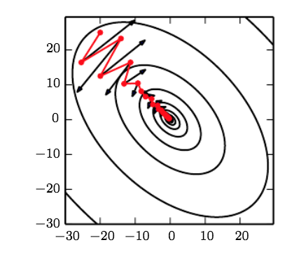
  • Momentum allows us to go "along the ravine" instead of "across the ravine", because we have influence from previous gradients. In the following pictures, regular SGD would have osciallted across the ravine but now we go down torwards the local minimum faster.

    

    Nesterov Momentum

• Variant of the momentum algorithm that consists of "taking the step" first in the direction of the momentum vector, and then "correcting" your parameters by the gradient there

  • Instead of the gradient where you currently are

• Updates:

  $$ v \leftarrow{} \alpha v - \epsilon \nabla_\theta \frac{1}{m}\sum_{i=1}^{m} L(f(x^i; \theta + \alpha v), y^i) $$

  $$ \theta \leftarrow{} \theta + v$$

• The main difference is that the gradient in nesterov momentum is evaulated after the parameters are adjusted by the (scaled) momentum factor, so we interpret this as adding a "correction" factor to the regular momentum method

Parameter Initialization Strategies

• Deep learning optimization: no convergence guaranted, several things affected by initial point, including whether the loss actually converges at all, and converges to a point with good generalizaiton error

  • Points of comparable cost can have wildly different results when tested (generalization error)

• Goal of initialization: have each unit compute a different function, in order to "break symmetry"

  • Need to break symmetry otherwise if each units have the same parameter values initially and are connected with the same inputs, the training process will cause them to be updated identically

• Weights generally initialized randomly from a Gaussian or Uniform distribution

• Scale of initialization is important to consider

  • Large weights: May result in more "symmetry-breaking" and may result in larger forward and backward pass signals initially, but at a cost:
    • Exploding gradients
    • "Chaos" in RNNs: extreme sensitivity to slight perturbations
    • Early saturation of certain activation functions (for example sigmoids)
  • Optimization suggests that we have larger weights (more signal to propagate information) while regularization encourages our weights to be smaller
  • Earlier it was shown that for some models, GD with early stopping is similar to $$L2$$ weight decay, and this provides an analogy of thinking of our parameter initializations as defining a prior distribution.
  • Concretely, we can think of initializing our params $\theta$ to $\theta_p$ to be imposing a Gaussian prior with mean $\mu = \theta_p$ on our model.
  • If we believe that our units don't interact with each other rather than they do interact, we should set $\theta_p = 0$. A large $\theta$ would mean that we have prior belief that our units do indeed interact with each other

• Glorot & Bengio's normal initialization:

  $$ W_{i,j} = U(-\sqrt{\frac{6}{m+n}}, \sqrt{\frac{6}{m+n}})$$ where $$ m$$ is the number of inputs into the layer and $$ n $$ is the number of outputs of the layer

  • This is meant to compromise between having the same activation variance and gradient variance
    • This is desired so that we don't have the "vanishing gradient" problem, and is similar to why we use batch normalization.

• Generally a good idea to treat the initial scale of the weights and hyperparameter search across it, as long as computational resources allow for this

• Another way to come up with a good weight initialization is to look at the activation and gradient variances of your model when a single batch of data is input.

  • If you see activations start to vanish, that's a good sign that you need to increase the value of your weights
  • If learning is still too slow, this will likely be indicated by vanish gradients in the backward pass

• Another common way to initialize parameters is by using unsupervised learning or supervised learning for a different task

  • Train for an unsupervised problem —> these parameters may encode information about the distribution of the training data, which may be better than random initalization

Adaptive Learning Rate Algorithms

• Learning rates are hard to set, and it has been shown that that the cost can sometimes be extremely sensitive to certain directions in the parameter space and insensitive to others. This motivates the desire for per-parameter learning rates

• AdaGrad

  • Adapt learning rates per-parameter

  • Each parameter's learning rate is scaled inverserly proportional by the square-rooted sum of all previous squared gradients

  • Parameters with large gradients therefore have smaller effective learning rates, and parameters with small gradients therefore have larger effective learning rates

  • Intuition: parameters with large gradients represent more intense curvature and changing directions across the optimization surface, while parameters with smaller gradients correspond to more consistent and gentle curvature. So we want to have larger gradient influence in the latter, while less in the former

  • A common criticism is that since it accumulates gradients from the start of training (when gradients are usually large) the algorithm decreases the effective learning rate too quickly to be effective

  • Update for Adagrad:

    Compute $$ g $$ as usual: $$ g = \frac{1}{m}\nabla_{\theta} \sum_{i=1}^{m} L(f(x^i ; \theta), y^i)$$

    Add $$ g$$ to the running squared gradient (here $$ r = 0$$ to begin with): $$ r = r + g \circ{}g$$ where $$ \circ$$ is the hadamard product

    Use $$ r $$ to scale the per-parameter learning rate for the update: $$ \theta = \theta - \frac{\epsilon}{\sqrt{\delta + r}}\circ{} g$$ where, per parameter, $$ \theta $$ is the weight to be updated, $$ \epsilon$$ is the global learning rate, $$ \delta$$ is a small constant for numerical stability, and $$ r $$ is the parameter's sum of squared gradients

    • The square root, division, and addition operations are applied elementwise, since $$ r $$ is a vector. Concretely, the operation $$ r = r + g \circ{} g $$ returns a vector, and each value in the vector represents the running sum of squared gradients of the particular parameter at that index. Therefore, this is the vectorized version of the algorithm - the term $$ \frac{\epsilon}{\sqrt{\delta + r}} $$ differs for each parameter, so each parameter is differently scaled, depending on the particular value of their sum of squared gradients.

    • As mentioned, if a particular parameter has a large sum of squared gradients, its gradient will be scaled relatively more, so a smaller step will be taken in that direction

    • We can see a clear downside with this: since the grads are generally large when learning begins, this approach may decrease the model's LR too quickly, and result in a model that is much slower to converge.

• RMSProp

  • AdaGrad had a problem: it weights all previous gradient updates equally, meaning that gradient updates far in the past have an equal influence on the effective learning rate that is computed as the current gradients do.

    • This may not be good, if we wish to adapt the individual parameter learning rates to the current optimization landscape we are at, as opposed to the optimization landscape in the past
    • Also, if there are large gradients in the past, then effective learning rates will always be small, and they will always continue to decrease
    • Example: AdaGrad is supposed to perform well in a convex bowl (it was originally designed for convex optimization), but it doesn't work if it was previously optimizing in a nonconvex landscape
    • Fix: RMSProp

  • RMSProp exponentially decays past learning rates, so that gradients from the past have much less of an influence on the current effective learning rate than present gradients. Our only difference is now that we introduce a decay variable $$ \rho$$ and scale our past squared gradient norms by this:

    $$ g = \frac{1}{m}\nabla_{\theta} \sum_{i=1}^{m} L(f(x^i ; \theta), y^i)$$

    $$ r = \rho r + (1 - \rho)g \circ g$$

    $$ \theta = \theta - \frac{\epsilon}{\sqrt{\delta + r}}\circ{}g$$

    • The square root, division, and addition operations are applied elementwise, similar to Adagrad. This update adjusts the learning rate per-parameter, making it so that each parameter's gradient is scaled by a per-parameter learning rate that is dependent on (exponentially decaying) past gradients.

    • A small value for $$ \rho$$ decreases the influence that past squared gradients have on the current effective learning rate, while a large value means that the past gradients should have a greater effect.

  • Note: A similar algorithm, AdaDelta, exists in order to resolve the same AdaGrad problem that RMSProp sought to solve. The solution is largely similar to that used in RMSProp, so the two algorithms are quite similar.

  • RMSProp is also commonly used with nesterov momentum; the two work together in the following manner:

    Evaluate $$ g $$ at the parameters offset by the momentum vector: $$ g = \frac{1}{m}\nabla_{\theta} \sum_{i=1}^{m} L(f(x^i ; \theta + \alpha v), y^i)$$

    Compute the effective learning rate in the same manner: $$ r = \rho r + (1 - \rho)g \circ g $$

    Update the momentum: $$ v = \alpha v - \frac{e}{\sqrt{\delta + r}}g$$

    Apply the update: $$ \theta = \theta + v $$

    ​

• Adam Optimizer - the most commonly used optimizer

  • Sort of combines RMSProp with momentum techniques - it keeps an exponentially decaying weighted average of past squared gradients, and an exponentially decaying weighted average of past gradients (similar to momentum)

  • Both of these constants are then adjusted for bias based on the current timestep, because since they are intialized to $$ 0$$, they are heavily biased towards $$ 0$$, especially at earlier timesteps and when the decay rates are close to $$ 1 $$. The algorithm:

    Let $$ s = 0 $$, $$ r = 0 $$, and keep track of the timestep $$ t $$, which is set to $$ 0 $$ as well.Now compute the gradient update:

    $$ g = \frac{1}{m}\nabla_{\theta} \sum_{i=1}^{m} L(f(x^i ; \theta), y^i)$$

    $$ t = t + 1 $$

    Update $$ s = \rho_1s + (1 - \rho_1)g $$ (exponentially decaying gradients, similar to momentum)

    Update $$  r = \rho_2 r + (1 - \rho_2)g \circ g$$ (exponentially squared decaying gradients, similar to RMSProp)

    Correct biases: $$ \hat{s} = \frac{s}{1 - \rho_1^t} $$ and $$ \hat{r} = \frac{r}{1 - \rho_2^t} $$ . Generally, $$ \rho $$ is large (between 0.9 and 0.999), so this will cause the biased estimates of the first and second moments to be large for lower timesteps (approximately being scaled by 100-1000ish x), and small for later timesteps (the limit is $$ r $$ or $$ s $$ itself as $$ t \rightarrow{} \infty $$.

    Perform update: $$ \theta = \theta - \epsilon \frac{\hat{s}}{\sqrt{\hat{r}}}$ \circ{} g$$

    Similar to above, this update will be per-parameter.

  • What does the update rule signify?

  • The authors call the term $$ \frac{\hat{s}}{\sqrt{\hat{r}}} $$ a "signal-to-noise ratio". If this ratio is close to $$ 0$$, this means that there is less certainty about $$ \hat{s} $$ corresponding to the direction of the true gradient, for example, this could occur near optimum, in which case smaller step sizes are good (so as to not overshoot the optimum, which could happen with a larger step size).

  • Why is there a bias adjustment?

  • Since $$ r $$ and $$ s $$ are initialized to $$ 0 $$, and the operations performed are additive, they are heavily biased to $$ 0 $$, especially at the beginning. The bias towards $$ 0 $$ is further contributed to by the fact that the decay constants $$ \rho $$ are usually around 0.99 (i.e. close to $$ 1 $$), so the decay is relatively slow. To fix this bias towards $$ 0 $$< the bias adjustments above are made, which make the values larger during earlier timesteps.

Second-Order Methods

• Newton's method - the main idea is to optimize the quadtratic approximation of the objective:

  $$ J(\theta) \approx J(\theta_0) + (\theta - \theta_0)^T\nabla_{\theta}J(\theta_0) + \frac{1}{2}(\theta - \theta_0)^T H (\theta - \theta_0) $$

• Solving for the critical point of the quadratic approximation gives us:

  $$ \theta = \theta_0 - H^{-1}\nabla_{\theta}J(\theta_0) $$ where $$ H $$ is the matrix of second derivatives evaluated at $$ \theta_0$$

• This term is similar to the usual Newton's method in single-variable calculus: $$ \theta = \theta_0 - \frac{f'(\theta_0)}{f''(\theta_0)} $$

• For a locally quadtratic function with positive-definite $$ H $$, Newton's method would immediately jump to the minimum. For a general convex optimization problem (with positive-definite $$ H $$) Newton's method can be applied iteratively to get to the global minimum.

• However, issues arise for nonconvex problems. As seen above, we simply solved for the approximation's critical point to determine where to jump, but this would only be a minima if we had convexity guarantees. In general, then, Newton's method will jump to a point with $$ 0 $$ gradient, which could also be a local max or saddle point. In this case, our algorithm would incorrectly conclude that it has converged, and make no more updates, even though it did not correctly find the minimum.

• As a fix for the above, in order to try to apply Newton's method to deep learning, we have the regularized Newton's method:

  $$ \theta = \theta_0 - (H + \alpha I)^{-1}\nabla_{\theta}J(\theta_0) $$ where $$ \alpha $$ is set to offset the magnitude of curvature in the optimization surface. For strong negative curvature, $$ \alpha $$ would need to be set to be very large, which could make Newton's method make such slow progress that regular first-order gradient methods would have optimized faster.

• The main limitation of using Newton's method in practice is complexity. If we have $$ k $$ params, then the Hessian is a $$ k * k $$ matrix, inversion of which is $$ O(k^3) $$, and considering that even small networks have millions of parameters, this is impractical.

Conjugate gradients method

• ​