Ch6-Feedforward-Neural-Networks.md

Chapter 6: Deep Feedforward Networks

Introduction

• Deep feedforward neural nets are also known as multilayer perceptrons
• Goal is to approximate a function $f*(x)$ by learning a mapping $y = f(x; \theta)$ where $\theta$ are the paramters to be learned by the model
• compose together many different functions, which can be represented by a DAG
• the final output of the model is called the output layer, while the intermediary layers are called hidden layers.

From linear models to neural networks

• One way to understand deep neural nets is by considering the limitations of linear models.
• Linear models are useful since they can fit data reliably and often have closed-form solutions or solutions that can be found via well-studied convex optimization techniques.
• However, they cannot represent nonlinear functions; in order to do this, we need to do a nonlinear feature transformation by applying a function $\phi$ to our inputs $x$.
• Idea is to have a learned representations $\phi(x)$.

Trying to learn XOR

• Our cost function is given by $$J(\theta) = \frac{1}{4} \sum_{x\in X} (f^*(x) - f(x;\theta))^2$$

• We can try to use a linear model of the form $$f(x; w, b) = x^Tw + b$$ and minimize the cost function $J$ with respect to $w$ and $b$. However, the optimal solution to this linear model is not able to solve the XOR problem; it just predicts $0.5$ everywhere.

• we fix this problem by using a nonlinear function. We usually apply an affine transformation the input of a layer followed by a nonlinear activiation function (Sigmoid, ReLu, tanh). In neural networks, we then take the result of this function and forward it through more hidden layers, and end with an affine transformation at the end.

ReLu

• default recommendation for nonlinearity in deep neural networks.

• Piecewise linear, but unable to learn when $x < 0$

• $f(x) = \max {0, x}$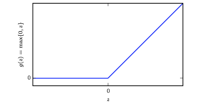

• Derivative of $f(x) = relu(x)$ with respect to input $x$ is $0$ when $x < 0$, and $1$ when $x > 0$. The gradient is technically undefined at $x = 0$, but is usually explicitly specified to be $0$.

• The complete formulation of the network with a single hidden layer is $f(x; W, c, w, b) = w^T\max(0, W^Tx + c) + b$

Gradient-Based Learning

• The nonlinearities involved with deep learning make gradient based learning more complicated.
• The loss functions are no longer convex, whereas convex optimization could reliably be used with linear models in order to obtain the optimal parameters, which find the global minimum of a cost function.
• On teh other hand, the cost function with respect to deep neural networks are not convex, so the best that gradient descent can do is reach a local minimum, and the solution is dependent on the initialization of the parameters.

Formulating Cost functions

• In most cases our model defines a distribution $p(y \mid x; \theta)$ and we simply use maximum likelihood - which corresponds to taking the cross-entropy loss as the cost function.
• Likelihood: $p(x_i, y_i \mid \theta) = p(y_i \mid x_i; \theta)p(x \mid \theta)$
• Data likelihood: $p(x_1, y_1 ... x_n y_n \mid \theta)$
• Expand & IID assumption: $p(x_1, y_1 \mid \theta) * ... p(x_n, y_n \mid \theta) = \prod_i p(y_i \mid x_i; \theta)$ (removing the $p(x_i \mid{} \theta)$ which the parameters do not influence)
• Negative log-likelihood: - $\sum_i \log p(y_i \mid x_i \theta)$
• If you set $p(y_i \mid x_i ; \theta) = N(y, f(x; \theta), I)$ then you recover the mean-squared loss.
• Neural nets are generally trained to maximize the data likelihood, which basically means the network should come up with a point estimate of the parameters $\theta$ that make observing the data most likely.
• $p(x)$
• Maximum likelihood maximizes $$p(D \mid \theta)$$ whereas MAP estimation maximizes $p(\theta \mid D)$
• $p(\theta \mid D) = \frac{p(D \mid \theta) * p(\theta)}{p(D)}$ but we generally discount the denominator since it is a normalization constant.
• Main difference is that with MAP the parameters are no longer a point estimate
• Many times CE cost does not have a minimum value when applied to models, but this can be mitigated through regularization.
• Generally, prefer to use the the CE loss instead of MSE or MAE (mean aboslute error)since using those loss functions with large networks and gradient-based learning results in saturation and very small gradients.
• For learning to occur, we require a large, predictable gradient to serve as a guide for the weight updates. This is why the choice of activation functions are important; activations such as sigmoid generally cause learning to slow down or completely stop because they are saturating nonlinearities , which means that their derivatives are zero at extreme values for the function.
• This is why the cross-entropy is commonly used as a cost function; it includes a $\log$ that undoes $\exp$ operations which could potentially cause saturation.

Output Units

Most times, we use the CE loss between the data distribution and the model distribution - as such, the output units we pick determines the from of the CE loss.

Assume $h = f(x, \theta)$.

Output activations

• The choice of output activations is important since we need to make sure that the gradients of these outputs are not frequently $0$, or else learning will not occur. For example, if we use the $CE$ loss with a ReLU ouput unit, the gradient of the output of the model with respect to the last layer will frequently be $0$, which when backpropagated, will result in no weight updates.
• Generally, use the sigmoid or softmax activations at the output of a network if you're optimizing the cross-entropy loss, otherwise have the outputs of your network just be the unchanged affine transformation.
• Sigmoid units can be used for Bernoulli output distributions, or binary classification.
• If we were to use a linear unit, then we would have to threshold it, which could lead to difficult gradients to train.
• One useful property of the softmax function is that $$ softmax(z) = softmax(z+c)$$, so we can avoid numerical computation problems by computing $$ softmax(z) = softmax(z- max_i{z_i})$$

Other Output Types

• If you want to learn the variance/covariance of a distribution, you can learn it as a parameter.
• Usually we use the perciscion, because the gradient is better behaved. WE usually only learn a diagonal percision/covariance matrix, as learning a full matrix requires $O(d^3)$ time.
• For multi-modal regression, we can use a Gaussian mixture model, which are particularly effective in speech generation.

Hidden Units

• Sigmoidal activation: $\sigma(x) = \frac{1}{1 + \exp(-x)}$.
• Derivative is $\sigma(x)(1 - \sigma(x))$.
• It behaves linearly around $x = 0$, and is everywhere differentiable. Also has the interpretation of a probability since the outputs are between $0$ and $1$, and also gives the "firing rate" of the neuron.
• Cons: Saturating gradient at extremes -> gradient is practically 0.
• max value of the gradient is $0.25$, so it also always scales down gradients as they are backpropagated through, which also can lead to the vanishing gradient problem.
• Another con is that it is centered around $0.5$, not $0$. This means that all of the outputs from the sigmoid neuron will be positive, and centered around $0.5$. This could result in "zig-zagging" during gradient descent. For concreteness, suppose that $f = \sum_i w_ix_i$ and $\frac{df}{dw_i} = x_i$. Then if we have a loss $L = \sum_i y^i - f(x^i)$, we have $\frac{dL}{dw_i} = \frac{dL}{df}\frac{df}{dw_i} = \frac{dL}{df}x_i$ This tells us that the gradient of the loss with respect to the weights will always have the same sign, since $x_i$ is positive, the gradients will either be all positive or all negative, resulting in "zig zagging" during gradient descent.
• Hyperbolic Tanh: $2\sigma(x) - 1$, $\frac{d}{dx}tanh(x) = 1 - tanh^2(x)$>
• This is still saturating but less so than the sigmoid, and behaves as a nearly linear unit for more of it's input range. Also has the property of beign zero-centerred, which means that there will not be much zig-zagging of the weight updates during gradient descent (see above for a more detailed description of this).

The Humble ReLU, and its several variations

• ReLU unit is given by $ReLU(x) = max(0, x)$. The local gradient is $1$ if $x > 0$ else $0$. The unit is not differentiable at $0$, but we generally assign a value to the derivative at $0$ between $0, 1$.
• The pros of the relu unit include faster convergence, behaves linearly when it's active, and does not scale gradients down during backpropagation, it rather just "passes them through" the unit.
• However, learning does not happen for examples with $0$ activation, which can lead to the "dying ReLU" problem which is when a ReLU neuron never activates, such as if its weights are not initialized properly or if a gradient update knocks them in a certain direction (literally what Karpathy's post says).
• The softplus unit $\log(1 + \exp(x))$ is a soft approximation of the ReLU who's derivative is the sigmoid function.
• The leaky relu seeks to solve teh dying ReLU problem by passing a smaller gradient when $x < 0$ and the unit is not active in teh forward pass. It is given by $\max(\alpha x, x)$ where $\alpha$ is a hyperparameter generally set to some small value like $0.01$. In the similar PReLU, this $\alpha$ is actually a parameter that can be optimized during learning.
• The exponential linear unit, or ELU, is another activation function that's designed to approximate the ReLU but also avoid teh stopping of learning when the unit is not active. It is given by $f(x) = \max(\alpha(\exp(x) - 1), x)$.

Output Activations

• Once we have the output socres form our network, we may want to run them through an activation function before calculating our loss or for interpretability purposes.
• A popular output activation is the sigmoid or more general softmax, which allows our scores to be interpreted as probabilities.
• Based on this, which loss function may be better to use? The MSE given by $L = \frac{1}{2}\sum_i (y^i - \sigma(z^i))$ or the cross entropy given by $l = -\sum_i y_i \log \sigma(z^i) + (1 - y_i)\log(1 - \sigma(z^i))$.
• If we consider the backwards pass, the derivatives are given by $-2(y_i - \sigma(z_i))\sigma'(z_i)$, so if $z$ is very large and negative or very large and positive, this gradient will be approximately zero. This isn't good because it implies that we have a lages loss and an inaccurate prediciton, but essentially zero gadient will be passed down to our weights, leading to extremely slow or nearly no learning (essentially the vanishing gradient problem again).
• On the other hand, the derivative for the cross entropy cost can be given by $\frac{dCE}{dz_i} = \sigma(z_i) - 1$, which is not dependent on the sigmoid derivative. In this case when $z$ is negative and large, then the gradient will have the highest magnitude, and it will only go towards zero when $z$ is positive and large, implying that we have a low loss, which makes sense.

Architecture Design

• Fully connected architecture: $h^1 = g^1(W^{1T}x + b^1)$ ... and so on, for however many layers that you have in the network
• Deeper networka generally have less units per layer and much fewere parameters, but generalize better, but are more computationally complex to train, and harder to optimize, because the vanishing/exploding gradient problem becomes more apparent.
• Universal Approximation Theorem states that a neural network with a single hidden layer with a nonlinearity can approximate any function. Essentially, we know that for any function that we are trying to learn, we know that there exists a setting of the params for the neural network such that we will be albe to represent that function, but this theorem says nothing about our ability to learn that function.
• This theorem does not really apply well in practice, because the hidden layer generally has to be extremely large and the training algorithm will overfit on the training dataset.

Alternatives to the fully connected architecture

• Convolutional networks only connect a limited number of neurons at each level.
• Recurrent networks make use of recurrent connections, sharing paramters across time. Skip connections in feedforward networks are also useful; they allow there to be connections from layer $i$ to for example layer $i + 3$, making it easier for the gradient to flow from output layer to earlier layers.

Backpropagation

• Method for computing the derivatives of a function $f$ with respect to f's inputs or parameters. For example, in machine learning, we generally use backpropagation to compute the gradient $\nabla_{\theta}J(\theta)$